Introduction
For the past 12 months, I've been building a research platform for training AI algorithms to learn Monopoly Deal via self-play. What began with humble aspirations to more closely study game theory and reinforcement learning has morphed into a clear data model, plug-and-play state abstractions, multiple training pipelines with multiple parallelization modes, and a polished web application for evaluation and interactive play. I even wrote a paper, Monopoly Deal: A Benchmark Environment for Bounded One-Sided Response Games, introducing Monopoly Deal as a novel benchmark for game-playing AI (mileage may vary, fingers crossed for a citation or two...). Honestly, it's been thrilling.
To date, I've only trained CFR models to learn this game. In this post, we turn to reinforcement learning: I train several policy-gradient models, compare them to CFR and to one another, and see how they perform.
Specifically, we train three models on two different state abstractions:
- Tabular REINFORCE
- Neural REINFORCE
- Neural Actor-Critic (GAE/PPO)
All models are trained with JAX and Optax on a single CPU. You can find the training code here, and play against these models at monopolydeal.ai. Below, we introduce each model, including the policy-gradient formulation, the generalized-advantage estimator, the PPO objective, the state abstractions, and the training modifications. Finally, we conclude with empirical results.
Policy Gradient
We begin with the standard episodic policy-gradient formulation. Define a single game trajectory as:
generated by a policy \(\pi_\theta(a\mid s)\). When training our model, we wish to maximize the expected return:
To achieve this goal, we'd like to tweak the policy parameters \(\theta\) in the direction of the gradient of \(J(\theta)\). Using the log-derivative trick, we can compute this gradient as:
where \(R_t = \sum_{k=t}^{T-1} r_k\) is the Monte Carlo return from timestep \(t\), i.e. the true return of the full trajectory.
Equivalently, we can write the gradient as \(\mathbb{E}_{\tau \sim \pi_\theta}\big[\nabla_\theta \log p_\theta(\tau)\, R(\tau)\big]\), which can be approximated with the unbiased estimator \(\frac{1}{N} \sum_{i=1}^N \nabla_\theta \log p_\theta(\tau_i)\, R(\tau_i)\), i.e. the sample average of the log-policy gradient times the true return. In this vein, actions that produce high returns are further encouraged, while actions followed by low returns are discouraged. This estimator is unbiased, easy to implement, and forms the basis of REINFORCE.
Unfortunately, in practice, this estimator's variance is high—especially in games with delayed terminal rewards, such as Monopoly Deal, with game lengths of ~50 turns—necessitating variance-reduction techniques. A common modification introduces a baseline \(b(s_t)\) that does not change the expectation:
Choosing \(b(s_t)\) to approximate the abstract value \(V(s_t)\) of the state—the trajectory reward expected if we follow the policy \(\pi_\theta\) from state \(s_t\)—yields the advantage, \(A_t = R_t - V(s_t)\). This is a simple measure that answers the question: "In this state, how much better is taking the specific action \(a_t\) than simply sampling from the policy itself?" This produces a modified gradient estimator, known as REINFORCE with a baseline.
However, this estimator still relies on the full Monte Carlo return \(R_t\), which sums random noise over the entire episode, resulting in high variance. To fix this, instead of using the full return, we bootstrap. We estimate the return using the immediate reward plus the discounted value of the next state: \(r_t + \gamma V(s_{t+1})\).
Relying on this predicted future reduces variance (since we don't sum noise over a long horizon) but introduces bias (since our value function might be wrong). Balancing this bias-variance trade-off is the core motivation behind Generalized Advantage Estimation (GAE).
Generalized Advantage Estimation
To more carefully control the bias-variance trade-off of the advantage estimator, Schulman et al. (2015) proposed Generalized Advantage Estimation (GAE), which replaces advantage estimates with a weighted average of \(n\)-step TD residuals.
Temporal-difference residuals
The one-step TD residual is
which provides a lower-variance (but biased) estimate of \(A_t\). Extending this to multi-step returns yields the \(n\)-step TD residual:
Small \(n\) produces low-variance but biased estimates; large \(n\) approaches the unbiased Monte Carlo return but comes with higher variance.
Exponential weighting
Generalized Advantage Estimation introduces an exponentially weighted mixture of these \(n\)-step estimators:
Equivalently, GAE can be written directly in terms of TD residuals (derivation in Equation 16 of the paper):
The parameters \(\gamma\) and \(\lambda\) play distinct roles in this estimation. \(\gamma\) is the discount factor, which is part of the problem definition itself; it determines the scale of the value function and how much the agent should care about long-term vs. immediate rewards. \(\lambda\), on the other hand, is a smoothing parameter used strictly for variance reduction.
The parameter \(\lambda\) allows us to interpolate between two extremes:
-
\(\lambda = 0\): This yields the standard one-step TD residual \(\delta_t = r_t + \gamma V(s_{t+1}) - V(s_t)\). It has the lowest variance but introduces bias, as it relies heavily on the accuracy of the current value function.
-
\(\lambda = 1\): This accumulates the full sum of discounted rewards. It is unbiased (assuming the correct \(\gamma\)) but suffers from high variance because it sums the noise of every step in the trajectory.
In our experiments, we did not perform extensive hyperparameter tuning, but found that \(\gamma=0.99\) and \(\lambda=0.9\) provided a reasonable balance, utilizing the value function to reduce variance while allowing real rewards to correct for value-function bias.
PPO
Although GAE provides stable advantage estimates, policy-gradient updates can still be unstable when the new policy diverges too quickly from the old one. Schulman et al. (2017) proposed Proximal Policy Optimization (PPO), which addresses this by constraining the size of each policy update through a clipped surrogate objective.
Given a batch of trajectories, let \(\pi_\theta\) be the current policy and \(\pi_{\theta_{\text{old}}}\) the policy used to generate the data. Define the probability ratio
A naïve policy-gradient update would directly maximize
However, this can create training instability when \(r_t(\theta)\) grows too large. PPO replaces this with a clipped objective:
The clipping enforces a bound on how far the policy can move in a single update, preventing extremely large or sign-flipping gradients when the policy changes too rapidly.
Value-function loss
In addition to our policy, we train a value function \(V_\theta(s)\) to predict the Monte Carlo return \(R_t\). This is done with a squared-error loss:
In our models, we use a shared encoder for the policy and value function. In practice, this simply means adding an additional logit in the model's output layer that, when passed through a sigmoid, predicts the eventual trajectory value.
Entropy regularization
Entropy regularization encourages the policy to remain exploratory:
where \(\mathcal{H}(\pi_\theta(\cdot \mid s_t))\) is the entropy of the policy at state \(s_t\). High entropy is useful early on; later it slows convergence. We therefore apply entropy decay, decreasing the entropy coefficient over training so the agent gradually shifts from exploration to refinement.
Combined objective
The full PPO loss used in this work is
where we minimize the total loss \(L(\theta)\), \(c_v\) is the value-loss weight, and \(c_e\) is the entropy coefficient. The optimization proceeds with multiple epochs over the same batch, yielding a more sample-efficient update while keeping the policy within the clipped "trust" region. The hyperparameters \(c_v\) and \(c_e\) are tuned to balance the influence of the value and entropy terms.
State Abstractions
The behavior of policy-gradient methods in Monopoly Deal is strongly shaped by the underlying state representation. Unlike CFR—where the abstraction defines the information sets over which regret is accumulated—policy-gradient models operate directly on a feature vector. The choice of abstraction therefore determines the dimensionality of the input, the required expressivity of the model, and the structure of the credit-assignment problem itself.
Intent-based abstraction
In the CFR paper, we use an "intent-based abstraction": instead of encoding raw card identities, it maps each game state to a structured summary of strategic “intents,” such as:
- Adding to a property set
- Completing a property set
- Collecting rent
- Giving cash to an opponent
- Giving a property to an opponent as cash
- Etc.
In practice, as this abstraction was designed by a human knowledgeable about the game, it is highly informative and produces competitive strategies with minimal memory overhead and fast convergence.
Full state abstraction
In this work, we also train on a full state representation. Rather than summarizing playability or intent, the state vector directly encodes:
- Counts of each raw card in the player's hand
- Counter of properties in the player's property set
- Counter of cash in the player's cash pile
- Counter of properties in the opponent's property set
- Counter of cash in the opponent's cash pile
This representation encodes maximal information about the game state. However, it requires the model to work significantly harder to learn the game's dynamics and strategic priorities. In theory, with enough training, we should expect the full state abstraction to outperform the intent abstraction.
Models We Train
Our experiments evaluate three policy-gradient models: Tabular REINFORCE, Neural REINFORCE, and Neural Actor-Critic (GAE/PPO). Each model is trained on the intent abstraction and the full state abstraction, yielding six total models. Within a model class, the same hyperparameters are used for both abstractions.
Tabular REINFORCE
For each abstract state–action pair, this model maintains a scalar logit and updates it with:
where \(R_t\) is the true Monte Carlo return from the timestep at which the action was taken. The dimensionality is small enough that a full table is feasible, and gradients act only on the logits of the visited state–action pairs. To compute action probabilities, we simply softmax the logits for the actions in a given state.
Neural REINFORCE
The neural REINFORCE model replaces the table with a small MLP producing action logits. Its training loop follows the same Monte Carlo policy-gradient update, but gradients now flow through shared weights and biases. This decouples states via generalization: the model can reason about actions in states it has never actually seen.
Neural Actor-Critic (GAE/PPO)
The Neural Actor-Critic (GAE/PPO) model uses a shared network for both the policy and value function. The policy is updated with the clipped PPO objective:
while the value network is trained with a squared-error loss on temporal-difference targets. Advantages \(A_t\) are computed using the generalized-advantage estimator.
Training setup
All three models are trained against a fixed CFR baseline. While CFR is guaranteed to converge to a Nash-optimal policy, the RL models are merely tasked with exploiting the CFR model itself. In addition, when the models reach a certain performance threshold against CFR, they are used as a "snapshot" model to self-play against themselves, discarding the CFR opponent outright.
All models are implemented in JAX and trained with Optax optimizers on a single CPU. Batching, rollout generation, advantage computation, and PPO epochs all run inside JIT-compiled functions.
Tricks to Get This to Train
Neural network models are notoriously "alchemical," and Monopoly Deal–with long episodes and sparse rewards—is a difficult game to learn! The following modifications were key for getting the neural network models to reliably converge on competitive policies.
Multiple epochs per update
The same rollout is reused for several gradient steps (10, in our experiments), providing more effective sample usage.
Shared policy–value parameters
The policy and value networks share a single encoder: the first few layers process the state and feed into both heads. This reduces parameter count, improves sample efficiency, and tends to stabilize value estimation early in training. (Unfortunately, we did not conduct strict ablations against other architectures, e.g. a separate head, and/or separate optimizer, for the policy and value functions.)
Entropy regularization and decay
An entropy bonus encourages the policy to remain exploratory:
High entropy is useful early on; later it slows convergence. We therefore apply entropy decay, decreasing \(\beta\) over training so the agent gradually shifts from exploration to refinement.
He initialization
Because the full state abstraction produces relatively high-dimensional inputs (card counts, property structures, cash values), careful initialization helps prevent early saturation. We initialize all dense layers with He uniform initialization (introduced in He et al. (2015)), which produced more stable early gradients than Xavier in this environment.
Learning-rate decay
Both REINFORCE and PPO models benefit from a decaying learning rate:
- Initial learning rate large enough to escape poor initial policies.
- Exponential decay to reduce variance in the late phase.
Value-loss weighting
The PPO objective includes a value-function regression term:
We tune \(c_v\) to balance the influence of the value head. If the weight is too small, the advantages become noisy; if too large, the model prioritizes value prediction at the expense of the policy.
Clip epsilon
The PPO ratio-clip parameter \(\epsilon\) is critical. Too small, and the policy barely moves; too large, and updates become unstable. Values between 0.1 and 0.3 consistently produced the most stable learning curves.
Gradient clipping
We apply global-norm gradient clipping to prevent noisy advantage estimates from generating outsized updates. This is especially important during the first few thousand steps before the value function stabilizes.
Batch size
Larger batch sizes (number of trajectories that comprise a given parameter update) reduce gradient variance and produce noticeably smoother training.
Full Hyperparameter Table
The following table summarizes the hyperparameters used when training each model.
| Model | Abstraction | Learning Rate | Hidden Layers | Epochs/Update | Batch Size | Entropy Coef | Value Loss Weight | Clip ε | γ | λ | Weight Decay | Gradient Clip | Entropy Decay | LR Decay | Games Trained |
|---|---|---|---|---|---|---|---|---|---|---|---|---|---|---|---|
| Tabular REINFORCE | Intent | 0.1 | — | 1 | 250 | — | — | — | — | — | — | — | — | — | 25000 |
| Tabular REINFORCE | Full | 0.1 | — | 1 | 250 | — | — | — | — | — | — | — | — | — | 25000 |
| Neural REINFORCE | Intent | 1e-3 | [256, 128] | 10 | 250 | — | — | — | — | — | 1e-5 | — | — | — | 25000 |
| Neural REINFORCE | Full | 1e-3 | [256, 128] | 10 | 250 | — | — | — | — | — | 1e-5 | — | — | — | 25000 |
| Neural Actor-Critic (GAE/PPO) | Intent | 5e-4 | [256, 128] | 10 | 250 | 0.02 | 1.0 | 0.1 | 0.99 | 0.9 | 1e-5 | 1.0 | — | — | 25000 |
| Neural Actor-Critic (GAE/PPO) | Full | 5e-4 | [256, 128] | 10 | 250 | 0.02 | 1.0 | 0.1 | 0.99 | 0.9 | 1e-5 | 1.0 | — | — | 25000 |
Experimental Setup
We train each model for 25,000 games. Initially, the model is trained against a fixed CFR baseline. Once the model reaches a certain performance threshold against CFR, it is used as a "snapshot" model to self-play against itself.
The models are evaluated every 250 games against the CFR baseline (as well as "random" and "risk-aware" heuristic opponents, not shown). During evaluation, each model uses an argmax policy, i.e. it always selects the action with the highest probability.
Below, we show the distribution of winrates against the CFR baseline in the final 10,000 games of training for each model.
Results

The results demonstrate that although the FullStateAbstraction contains more information, and therefore should be more powerful, the IntentStateAbstraction produces more competitive policies across all models. This is likely due to the fact that the IntentStateAbstraction encodes the game's strategic priorities outright, significantly simplifying the learning problem.
Slicing by abstraction type, we see that for the FullStateAbstraction, performance improves as the model becomes more complex, with the Neural Actor-Critic (GAE/PPO) model achieving the highest performance. Conversely, for the IntentStateAbstraction, the Neural REINFORCE model achieves the highest performance. We hypothesize that the IntentStateAbstraction creates a smoother optimization landscape where PPO's conservative trust-region constraints are unnecessary, allowing the more aggressive REINFORCE updates to converge faster.
Overall, the results demonstrate that a medium-complexity neural network model that can generalize across unseen states, combined with an intent-based state abstraction that encodes a useful learning manifold a priori, produces the most competitive policy.
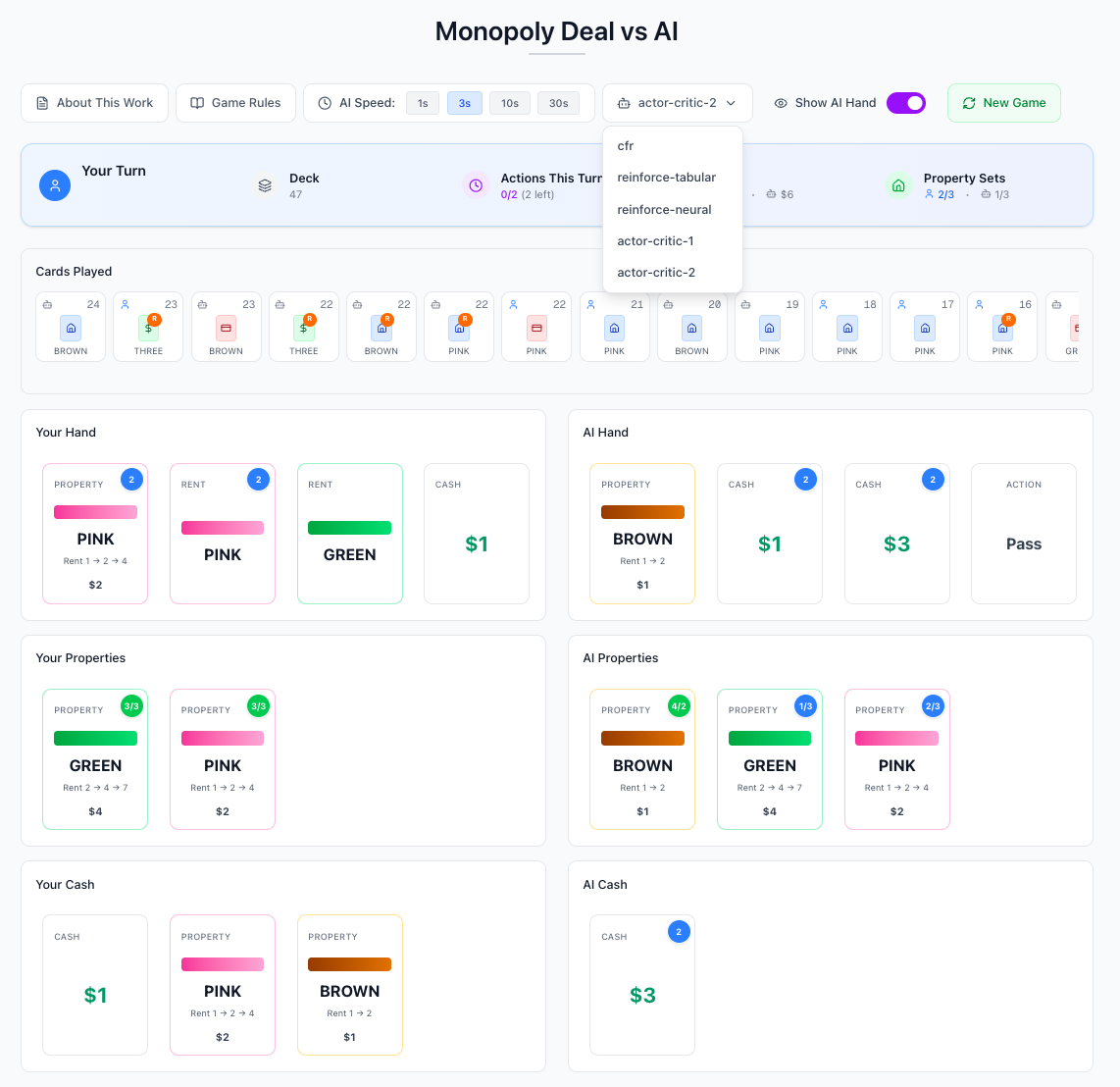
If interested, you can play against these models at monopolydeal.ai and see for yourself.
Conclusion
In this post, we trained three policy-gradient models on two different state abstractions: IntentStateAbstraction and FullStateAbstraction. We found that the IntentStateAbstraction produces more competitive policies across all models, and that a medium-complexity neural network model that can generalize across unseen states, combined with an intent-based state abstraction that encodes the game's key strategic priorities, produces the most competitive policy.
Acknowledgments
I'd like to thank Carey Hughes for introducing me to the game of Monopoly Deal last summer.