Bayesian inference is the task of quantifying a posterior belief over parameters $\boldsymbol{\theta}$ given observed data $\mathbf{x}$—where $\mathbf{x}$ was generated from a model $p(\mathbf{x}\mid{\boldsymbol{\theta}})$—via Bayes' Theorem:

$$ p(\boldsymbol{\theta}\mid\mathbf{x}) = \frac{p(\mathbf{x}\mid\boldsymbol{\theta})p(\boldsymbol{\theta})}{p(\mathbf{x})} $$

In numerous applications of scientific interest, e.g. cosmological, climatic or urban-mobility phenomena, the likelihood of the data $\mathbf{x}$ under the data-generating function $p(\mathbf{x}\mid\boldsymbol{\theta})$ is intractable to compute, precluding classical inference approaches. Notwithstanding, simulating new data $\mathbf{x}$ from this function is often trivial—for example, by coding the generative process in a few lines of Python—

def generative_process(params):
    data = ...  # some deterministic logic
    data = ...  # some stochastic logic
    data = ...  # whatever you want!
    return data

simulated_data = [generative_process(p) for p in [.2, .4, .6, .8, 1]]

—motivating the study of simulation-based Bayesian inference methods, termed SBI.

Furthermore, the evidence $p(\mathbf{x}) = \int{p(\mathbf{x}\mid\boldsymbol{\theta})p(\boldsymbol{\theta})}d\boldsymbol{\theta}$ is typically intractable to compute as well. This is because the integral has no closed-form solution; or, were the functional form of the likelihood (which we don't have) and the prior (which we do have) available, expanding these terms yields a summation over an "impractically large" number of terms, e.g. the number of possible cluster assignment configurations in a mixture of Gaussians (Blei et al., 2017). For this reason, in SBI, we typically estimate the unnormalized posterior $\tilde{p}(\boldsymbol{\theta}\mid\mathbf{x}) = p(\mathbf{x}\mid\boldsymbol{\theta})p(\boldsymbol{\theta}) \propto \frac{p(\mathbf{x}\mid\boldsymbol{\theta})p(\boldsymbol{\theta})}{p(\mathbf{x})}$.

Recent work has explored the use of neural networks to perform key density estimation tasks, i.e. subroutines, of the SBI routine itself. We refer to this work as Neural SBI. In the following sections, we detail the various classes of these estimation tasks. For a more thorough analysis of their respective motivations, behaviors, and tradeoffs, we refer the reader to the original work.

Neural Posterior Estimation

In this class of models, we estimate $\tilde{p}(\boldsymbol{\theta}\mid\mathbf{x})$ with a conditional neural density estimator $q_{\phi}(\boldsymbol{\theta}\mid\mathbf{x})$. Simply, this estimator is a neural network with parameters $\phi$ that accepts $\mathbf{x}$ as input and produces $\boldsymbol{\theta}$ as output. For example, It is trained on data tuples $\{\boldsymbol{\theta}_n, \mathbf{x}_n\}_{1:N}$ sampled from $p(\mathbf{x}, \boldsymbol{\theta}) = p(\mathbf{x}\mid\boldsymbol{\theta})p(\boldsymbol{\theta})$, where $p(\boldsymbol{\theta})$ is a prior we choose, and $p(\mathbf{x}\mid\boldsymbol{\theta})$ is our simulator. For example, we can construct this training set as follows:

data = []

for _ in range(N_SAMPLES):
    theta = prior.sample()
    x = generative_process(theta)

    data.append((x, theta))

Then, we train our network.

q_phi.train(data)

Finally, once trained, we can estimate $\tilde{p}(\boldsymbol{\theta}\mid\mathbf{x} = \mathbf{x}_o)$—our posterior belief over parameters $\boldsymbol{\theta}$ given our observed (not simulated!) data $\mathbf{x}_o$ as $\tilde{p}(\boldsymbol{\theta}\mid\mathbf{x}_o) = q_{\phi}(\boldsymbol{\theta}\mid\mathbf{x} = \mathbf{x}_o)$.

Learning the wrong estimator

Ultimately, our goal is to perform the following computation:

$$ q_{\phi}(\boldsymbol{\theta}\mid\mathbf{x} = \mathbf{x}_o) $$

Such that $q_{\phi}$ produces an accurate estimation of the parameters $\boldsymbol{\theta}$ given observed data $\mathbf{x}_o$, we require that $q_{\phi}$ be trained on tuples $\{\boldsymbol{\theta}_n, \mathbf{x}_n\}$ where:

$\mathbf{x}_n \sim p(\mathbf{x}\mid\boldsymbol{\theta}_n)$ via our simulation step.
$\mid\mathbf{x}_n - \mathbf{x}_o\mid$ is small, i.e. our simulated are nearby our observed data.

Otherwise, $q_{\phi}$ will learn to estimate a posterior over parameters given data unlike our own.

Learning a better estimator

So, how do we obtain parameters $\boldsymbol{\theta}_n$ that produce $\mathbf{x}_n \sim p(\mathbf{x}\mid\boldsymbol{\theta}_n)$ near $\mathbf{x}_o$? We take those that have high (estimated) posterior density given $\mathbf{x}_o$!

In this vein, we build our training set as follows:

data = []

for _ in range(N_SAMPLES):
    theta = q_phi(x=x_o).sample()
    x = generative_process(theta)

    data.append((x, theta))

Stitching this all together, our SBI routine becomes:

for r in range(N_ROUNDS):
    data = []
    for _ in range(N_SAMPLES):
        if r == 0:
            theta = prior.sample()
        else:
            theta = q_phi(x=x_o).sample()
        x = generative_process(theta)

        data.append((x, theta))
    q_phi.train(data)

posterior_samples = [q_phi(x=x_o).sample() for _ in range(ANY_NUMBER)]

Learning the right estimator

Unfortunately, we're still left with a problem:

In the first round, we learn $q_{\phi, r=0}(\boldsymbol{\theta}\mid\mathbf{x}) \approx p(\mathbf{x}\mid\boldsymbol{\theta})p(\boldsymbol{\theta})$, i.e. the right estimator.
Thereafter, we learn $q_{\phi, r}(\boldsymbol{\theta}\mid\mathbf{x}) \approx p(\mathbf{x}\mid\boldsymbol{\theta})q_{\phi, r-1}(\boldsymbol{\theta}\mid\mathbf{x})$, i.e. the wrong estimator.

So, how do we correct this mistake?

In Papamakarios and Murray (2016), the authors adjust the learned posterior $q_{\phi, r}(\boldsymbol{\theta}\mid\mathbf{x})$ by simply dividing it by $q_{\phi, r-1}(\boldsymbol{\theta}\mid\mathbf{x})$ then multiplying it by $p(\boldsymbol{\theta})$. Furthermore, as they choose $q_{\phi}$ to be a Mixture Density Network—a neural network which outputs the parameters of a mixture of Gaussians—and the prior to be "simple distribution (uniform or Gaussian, as is typically the case in practice)," this adjustment can be done analytically.

Conversely, Lueckmann et al. (2017) train $q_{\phi}$ on a target reweighted to similar effect: instead of maximizing the total (log) likelihood $\Sigma_{n} \log q_{\phi}(\boldsymbol{\theta}_n\mid\mathbf{x}_n)$, they maximize $\Sigma_{n} \log w_n q_{\phi}(\boldsymbol{\theta}_n\mid\mathbf{x}_n)$, where $w_n = \frac{p(\boldsymbol{\theta}_n)}{q_{\phi, r-1}(\boldsymbol{\theta}_n\mid\mathbf{x}_n)}$.

While both approaches carry further nuance and potential pitfalls, they bring us effective methods for using a neural network to directly estimate a faithful posterior in SBI routines.

Neural Likelihood Estimation

In neural likelihood estimation (NLE), we use a neural network to directly estimate the (intractable) likelihood function of the simulator $p(\mathbf{x}\mid\boldsymbol{\theta})$ itself. We denote this estimator $q_{\phi}(\mathbf{x}\mid\boldsymbol{\theta})$. Finally, we compute our desired posterior as $\tilde{p}(\boldsymbol{\theta}\mid\mathbf{x}_o) \approx q_{\phi}(\mathbf{x}_o\mid\boldsymbol{\theta})p(\boldsymbol{\theta})$.

Similar to Neural Posterior Estimation (NPE) approaches, we'd like to learn our estimator on inputs $\boldsymbol{\theta}$ that produce $\mathbf{x}_n \sim p(\mathbf{x}\mid\boldsymbol{\theta}_n)$ near $\mathbf{x}_o$. To do this, we again sample them from regions of high approximate posterior density. In each round $r$, in NPE, this posterior was $q_{\phi, r-1}(\boldsymbol{\theta}\mid\mathbf{x} = \mathbf{x}_o)$; in NLE, it is $q_{\phi, r-1}(\mathbf{x}_o\mid\boldsymbol{\theta})p(\boldsymbol{\theta})$. In both cases, we draw samples from our approximate posterior density, then feed them to the simulator to generate novel data for training our estimator $q_{\phi, r}$.

For a more detailed treatment, please refer to original works Papamakarios et al. (2019) and Lueckmann et al. (2019) (among others).

Neural Likelihood Ratio Estimation

In this final class of models, we instead try to directly draw samples from the true posterior itself. However, since we can't compute $p(\mathbf{x}\mid\boldsymbol{\theta})$ nor $p(\mathbf{x})$, we first need a sampling algorithm that satisifes these constraints. One such class of algorithms is Markov chain Monte Carlo, termed MCMC.

In MCMC, we first propose parameter samples $\boldsymbol{\theta}_i$ from a proposal distribution. Then, we evaluate their fitness by asking the question: "does this sample $\boldsymbol{\theta}_i$ have higher posterior density than the previous sample $\boldsymbol{\theta}_j$ we drew?" Generally, this question is answered through comparison, e.g.

$$ \frac{ p(\boldsymbol{\theta}_i\mid\mathbf{x}) } { p(\boldsymbol{\theta}_{j}\mid\mathbf{x}) } = \frac{ p(\mathbf{x}\mid\boldsymbol{\theta}_i)p(\boldsymbol{\theta}_i) / p(\mathbf{x}) } { p(\mathbf{x}\mid\boldsymbol{\theta}_j)p(\boldsymbol{\theta}_j) / p(\mathbf{x}) } $$

Fortunately, the evidence terms $p(\mathbf{x})$ cancel, and the prior densities $p(\boldsymbol{\theta})$ are evaluable. Though we cannot compute the likelihood terms outright, we can estimate their ratio and proceed with MCMC as per normal. If $\frac{p(\boldsymbol{\theta}_i\mid\mathbf{x})}{p(\boldsymbol{\theta}_j\mid\mathbf{x})} \gt 1$, we (are likely to) accept $\boldsymbol{\theta}_i$ as a valid sample from our target posterior.

Estimating the likelihood ratio

Let us term the likelihood ratio as

$$ r(\mathbf{x}\mid\boldsymbol{\theta}_i, \boldsymbol{\theta}_j) = \frac{ p(\mathbf{x}\mid\boldsymbol{\theta}_i) } { p(\mathbf{x}\mid\boldsymbol{\theta}_j) } $$

Ingeniously, Cranmer et al. (2015) propose to learn a classifier to discriminate samples $\mathbf{x} \sim p(\mathbf{x}\mid\boldsymbol{\theta}_i)$ from $\mathbf{x} \sim p(\mathbf{x}\mid\boldsymbol{\theta}_j)$, then use its predictions to estimate $r(\mathbf{x}\mid\boldsymbol{\theta}_i, \boldsymbol{\theta}_j)$.

To do this, they draw training samples $(\mathbf{x}, y=1) \sim p(\mathbf{x}\mid\boldsymbol{\theta}_i)$ and $(\mathbf{x}, y=0) \sim p(\mathbf{x}\mid\boldsymbol{\theta}_j)$ then train a binary classifer $d(y\mid\mathbf{x})$ on this data. In this vein, a perfect classifier gives:

$$ \begin{align*} d^*(y=1\mid\mathbf{x}) &= \frac{ p(\mathbf{x}\mid\boldsymbol{\theta}_i) } { p(\mathbf{x}\mid\boldsymbol{\theta}_i) + p(\mathbf{x}\mid\boldsymbol{\theta}_j) } \\ d^*(y=0\mid\mathbf{x}) &= \frac{ p(\mathbf{x}\mid\boldsymbol{\theta}_j) } { p(\mathbf{x}\mid\boldsymbol{\theta}_i) + p(\mathbf{x}\mid\boldsymbol{\theta}_j) } \\ \end{align*} $$

Consequently,

$$ \begin{align*} r(\mathbf{x}\mid\boldsymbol{\theta}_i, \boldsymbol{\theta}_j) &= \frac{ p(\mathbf{x}\mid\boldsymbol{\theta}_i) } { p(\mathbf{x}\mid\boldsymbol{\theta}_j) } \\ &= \frac{ d^*(y=1\mid\mathbf{x}) } { d^*(y=0\mid\mathbf{x}) } \\ &= \frac{ d^*(y=1\mid\mathbf{x}) } { 1 - d^*(y=1\mid\mathbf{x}) } \end{align*} $$

Since our classifier won't be perfect, we simply term it $d(y\mid\mathbf{x})$, where

$$ \begin{align*} \hat{r}(\mathbf{x}\mid\boldsymbol{\theta}_i, \boldsymbol{\theta}_j) &= \frac{d(y=1\mid\mathbf{x})}{1 - d(y=1\mid\mathbf{x})}\\ &\approx r(\mathbf{x}\mid\boldsymbol{\theta}_i, \boldsymbol{\theta}_j) \end{align*} $$

With $\hat{r}(\mathbf{x}\mid\boldsymbol{\theta}_i, \boldsymbol{\theta}_j)$ in hand, we can compare the posterior density of proposed samples $\boldsymbol{\theta}_i$ and $\boldsymbol{\theta}_j$ in our MCMC routine.

Generalizing our classifier

To use the above classifier in our inference routine, we must retrain a new classifier for every unique set of parameters $\{\boldsymbol{\theta}_i, \boldsymbol{\theta}_j\}$. Clearly, this is extremely impractical. How can we generalize our classifier such that we only have to train it once?

In Cranmer et al. (2015), the authors learn a single classifier $d(y\mid\mathbf{x}, \boldsymbol{\theta})$ to discriminate samples $\mathbf{x} \sim p(\mathbf{x}\mid\boldsymbol{\theta})$ from $\mathbf{x} \sim p(\mathbf{x}\mid\boldsymbol{\theta}_{ref})$, where $\boldsymbol{\theta}$ is an arbitrary parameter value, and $\boldsymbol{\theta}_{ref}$ is a fixed, reference parameter value. It is trained on data $(\mathbf{x}, \boldsymbol{\theta}, y=1) \sim p(\mathbf{x}\mid\boldsymbol{\theta})$ and $(\mathbf{x}, \boldsymbol{\theta}_{ref}, y=0) \sim p(\mathbf{x}\mid\boldsymbol{\theta}_{ref})$. Once trained, it gives:

$$ r(\mathbf{x}\mid\boldsymbol{\theta}, \boldsymbol{\theta}_{ref}) = \frac{ d^*(y\mid\mathbf{x}, \boldsymbol{\theta}) } { 1 - d^*(y\mid\mathbf{x}, \boldsymbol{\theta}) } $$

Consequently,

$$ \begin{align*} r(\mathbf{x}\mid\boldsymbol{\theta}_i, \boldsymbol{\theta}_j) &= \frac{ r(\mathbf{x}\mid\boldsymbol{\theta}_i, \boldsymbol{\theta}_{ref}) } { r(\mathbf{x}\mid\boldsymbol{\theta}_j, \boldsymbol{\theta}_{ref}) } \\ &= \frac{ d^*(y\mid\mathbf{x}, \boldsymbol{\theta}_i) } { 1 - d^*(y\mid\mathbf{x}, \boldsymbol{\theta}_i) } * \frac{ 1 - d^*(y\mid\mathbf{x}, \boldsymbol{\theta}_j) } { d^*(y\mid\mathbf{x}, \boldsymbol{\theta}_j) } \end{align*} $$

With a single model, we can now compare the density of two proposed posterior samples.

Improving our generalized classifier

Once more, our classifier $d(y\mid\mathbf{x}, \boldsymbol{\theta})$ discriminates samples $\mathbf{x} \sim p(\mathbf{x}\mid\boldsymbol{\theta})$ from $\mathbf{x} \sim p(\mathbf{x}\mid\boldsymbol{\theta}_{ref})$. In this vein, in the case that a given $\mathbf{x}$ was drawn from neither $p(\mathbf{x}\mid\boldsymbol{\theta})$ nor $p(\mathbf{x}\mid\boldsymbol{\theta}_{ref})$, what should our classifier do? In Hermans et al. (2019), the authors illustrate this problem—

png

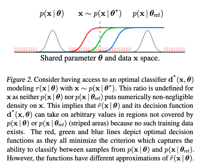
—stressing that "poor inference results occur in the absence of support between $p(\mathbf{x}\mid\boldsymbol{\theta})$ and $p(\mathbf{x}\mid\boldsymbol{\theta}_{ref})$."

In solution, they propose to learn a (neural) classifier that instead discriminates between dependent sample-parameter pairs $(\mathbf{x}, \boldsymbol{\theta}) \sim p(\mathbf{x}\mid\boldsymbol{\theta})p(\boldsymbol{\theta})$ from independent sample-parameter pairs $(\mathbf{x}, \boldsymbol{\theta}) \sim p(\mathbf{x})p(\boldsymbol{\theta})$. Since $p(\mathbf{x}\mid\boldsymbol{\theta})p(\boldsymbol{\theta})$ and $p(\mathbf{x})p(\boldsymbol{\theta})$ occupy the same space, they share a common support. In other words, the likelihood of a given $\mathbf{x}$ will always be positive for some $\boldsymbol{\theta}$ in the figure above.

Conclusion

Simulation-based inference is a class of techniques that allows us to perform Bayesian inference where our data-generating model $p(\mathbf{x}\mid\boldsymbol{\theta})$ lacks a tractable likelihood function, yet permits simulation of novel data. In the above sections, we detailed several SBI approaches, and ways in which neural networks are currently being used in each.

Credit

Credit to ProcessMaker for social card image.

Bibliography

David M. Blei, Alp Kucukelbir, and Jon D. McAuliffe. Variational Inference: A Review for Statisticians. Journal of the American Statistical Association, 112(518):859–877, 2017. arXiv:1601.00670, doi:10.1080/01621459.2017.1285773. ↩

Kyle Cranmer, Juan Pavez, and Gilles Louppe. Approximating Likelihood Ratios with Calibrated Discriminative Classifiers. arXiv, 2015. arXiv:1506.02169. ↩ ¹ ²

Joeri Hermans, Volodimir Begy, and Gilles Louppe. Likelihood-free MCMC with Amortized Approximate Ratio Estimators. arXiv, 2019. arXiv:1903.04057. ↩

Jan-Matthis Lueckmann, Giacomo Bassetto, Theofanis Karaletsos, and Jakob H. Macke. Likelihood-free inference with emulator networks. In Francisco Ruiz, Cheng Zhang, Dawen Liang, and Thang Bui, editors, Proceedings of The 1st Symposium on Advances in Approximate Bayesian Inference, volume 96 of Proceedings of Machine Learning Research, 32–53. 02 Dec 2019. PMLR. URL: http://proceedings.mlr.press/v96/lueckmann19a.html. ↩

Jan-Matthis Lueckmann, Pedro J Goncalves, Giacomo Bassetto, Kaan Öcal, Marcel Nonnenmacher, and Jakob H Macke. Flexible statistical inference for mechanistic models of neural dynamics. arXiv, 2017. arXiv:1711.01861. ↩

George Papamakarios and Iain Murray. Fast ε-free inference of simulation models with bayesian conditional density estimation. In D. Lee, M. Sugiyama, U. Luxburg, I. Guyon, and R. Garnett, editors, Advances in Neural Information Processing Systems, volume 29. Curran Associates, Inc., 2016. URL: https://proceedings.neurips.cc/paper/2016/file/6aca97005c68f1206823815f66102863-Paper.pdf. ↩

George Papamakarios, David Sterratt, and Iain Murray. Sequential neural likelihood: fast likelihood-free inference with autoregressive flows. In Kamalika Chaudhuri and Masashi Sugiyama, editors, Proceedings of the Twenty-Second International Conference on Artificial Intelligence and Statistics, volume 89 of Proceedings of Machine Learning Research, 837–848. PMLR, 16–18 Apr 2019. URL: http://proceedings.mlr.press/v89/papamakarios19a.html. ↩

Neural Methods in Simulation-Based Inference

Will Wolf