Most introductory tutorials on Gaussian processes start with a nose-punch of statements, like:

A Gaussian process (GP) defines a distribution over functions.
A Gaussian process is non-parametric, i.e. it has an infinite number of parameters (duh?).
Marginalizing a Gaussian over a subset of its elements gives another Gaussian.
Conditioning a subset of the elements of a Gaussian on another subset of its elements gives another Gaussian.

They continue with terms, like:

Kernels
Posterior over functions
Squared-exponentials
Covariances

Alas, this is often confusing to the GP beginner; the following is the introductory tutorial on GPs that I wish I'd had myself.

By the end of this tutorial, you should understand:

What a Gaussian process is and how to build one in NumPy.
The motivations behind their functional form, i.e. how the GP comes to be.
The statements and terms above.

Let's get started.

Playing with Gaussians

Before moving within 500 nautical miles of the Gaussian process, we're going to start with something far easier: vanilla Gaussians themselves. This will help us to build intuition. We'll arrive at the GP before you realize.

The Gaussian distribution, a.k.a. the Normal distribution, can be thought of as a Python object which:

Is instantiated with characteristic parameters mu (the mean) and var (the variance).
Has a single public method, density, which accepts a float value x, and returns a float proportional to the probability of this Gaussian having produced x.

class Gaussian:

    def __init__(self, mu, var):
        self.mu = mu
        self.var = var
        self.stddev = np.sqrt(var)  # the standard deviation is the square-root of the variance

    def density(self, x):
        return norm(loc=self.mu, scale=self.stddev).pdf(x)

So, how do we make those cool bell-shaped plots? A 2D plot is just a list of tuples— each with an x, and a corresponding y—shown visually.

As such, we lay out our x-axis, then compute the corresponding y—the density—for each. We'll choose an arbitrary mu and variance.

gaussian = Gaussian(mu=.123, var=.456)

x = np.linspace(-5, 5, 100)
y = [gaussian.density(xx) for xx in x]

plt.figure(figsize=(8, 5))
plt.plot(x, y)
_ = plt.title('`Gaussian(mu=.123, var=.456)` Density')

png

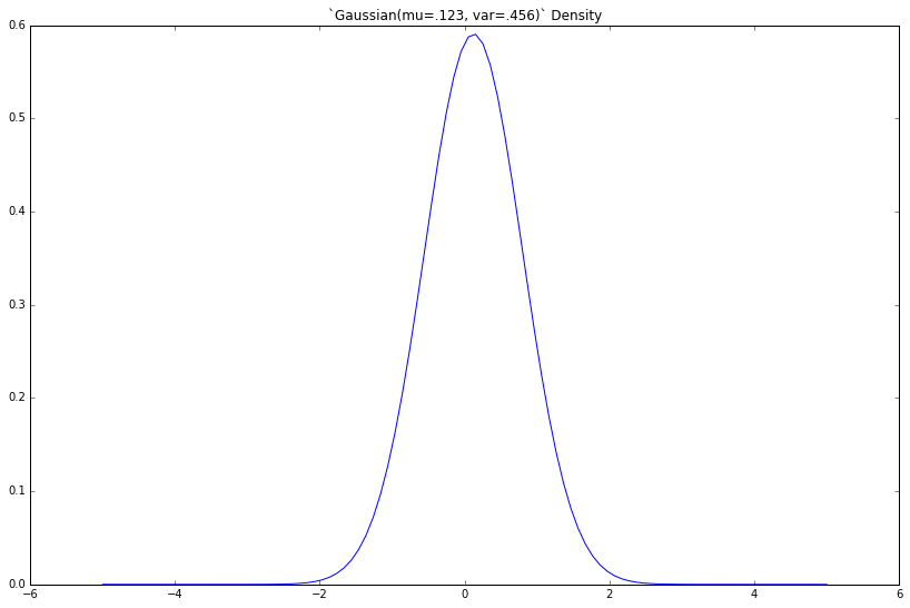
If we increase the variance var, what happens?

bigger_number = 3.45

gaussian = Gaussian(mu=.123, var=bigger_number)

x = np.linspace(-5, 5, 100)
y = [gaussian.density(xx) for xx in x]

plt.figure(figsize=(8, 5))
plt.plot(x, y)
_ = plt.title('`Gaussian(mu=.123, var=bigger_number)` Density')

png

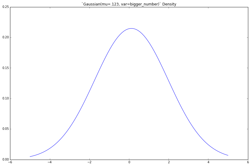
The density gets fatter. This should be familiar to you.

Similarly, we can draw samples from a Gaussian distribution, e.g. from the initial Gaussian(mu=.123, var=.456) above. Its corresponding density plot (also above) governs this procedure, where (x, y) tuples give the (unnormalized) probability y that a given sample will take the value x.

x-values with large corresponding y-values are more likely to be sampled. Here, values near .123 are most likely to be sampled.

Let's add a method to our class, draw 500 samples, then plot their histogram.

def sample(self):
    return norm(loc=self.mu, scale=self.stddev).rvs()


# Add method to class
Gaussian.sample = sample

# Instantiate new Gaussian
gaussian = Gaussian(mu=.123, var=.456)

# Draw samples
samples = [gaussian.sample() for _ in range(500)]

# Plot
plt.figure(figsize=(8, 5))
pd.Series(samples).hist(grid=False, bins=15)
_ = plt.title('Histogram of 500 samples from `Gaussian(mu=.123, var=.456)`')

png

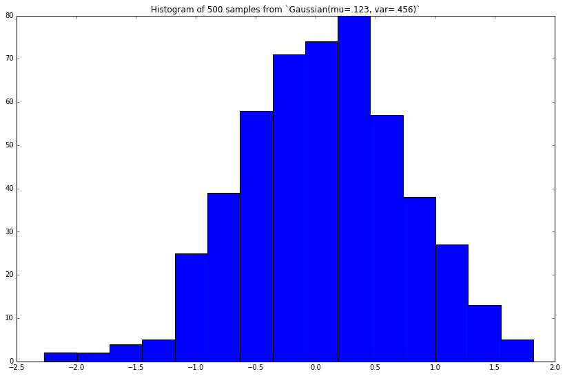
This looks similar to the true Gaussian(mu=.123, var=.456) density we plotted above. The more random samples we draw (then plot), the closer this histogram will approximate the true density.

Now, we'll start to move a bit faster.

2D Gaussians

We just drew samples from a 1-dimensional Gaussian, i.e. the sample itself was a single float. The parameter mu dictated the most-likely value for the sample to assume, and the variance var dictated how much these sample-values vary (hence the name variance).

>>> gaussian.sample()
-0.5743030051553177
>>> gaussian.sample()
0.06160509014194515
>>> gaussian.sample()
1.050830033400354

In 2D, each sample will be a list of two numbers. mu will dictate the most-likely pair of values for the sample to assume, and a second parameter (yet unnamed) will dictate:

How much the values for the first element of the pair vary
How much the values for the second element of the pair vary
How much the first and second elements vary with each other, e.g. if the first element is larger than expected (i.e. larger than its corresponding mean), to what extent does the second element "follow suit" (and assume a value larger than expected as well)

The second parameter is the covariance matrix, cov. The elements on the diagonal give Items 1 and 2. The elements off the diagonal give Item 3. The covariance matrix is always square, and the values along its diagonal are always non-negative.

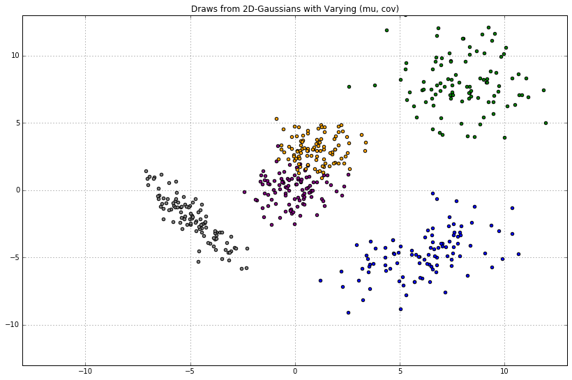
Given a 2D mu and 2x2 cov, we can draw samples from the 2D Gaussian. Here, we'll use NumPy. Inline, we comment on the expected shape of the samples.

plt.figure(figsize=(11, 7))
plt.ylim(-13, 13)
plt.xlim(-13, 13)


def plot_2d_draws(mu, cov, color, n_draws=100):
    x, y = zip(*[np.random.multivariate_normal(mu, cov) for _ in range(n_draws)])
    plt.scatter(x, y, c=color)


"""
The purple dots should center around `(x, y) = (0, 0)`.

`np.diag([1, 1])` gives the covariance matrix `[[1, 0], [0, 1]]`:

`x`-values have a variance of `var=1`;
`y`-values have `var=1`;
these values do not covary with one another.
"""
plot_2d_draws(
    mu=np.array([0, 0]),
    cov=np.diag([1, 1]),
    color='purple'
)

"""
The blue dots should center around `(x, y) = (1, 3)`. Same story with the covariance.
"""
plot_2d_draws(
    mu=np.array([1, 3]),
    cov=np.diag([1, 1]),
    color='orange'
)

"""
Here, the values along the diagonal of the covariance matrix are much larger:

the cloud of green points should be much more disperse.

There is no off-diagonal covariance.
"""
plot_2d_draws(
    mu=np.array([8, 8]),
    cov=np.diag([4, 4]),
    color='green'
)

"""
The covariance matrix has off-diagonal values of -2.

This means that if `x` trends above its mean, `y` will tend to vary *twice as much, below its mean.*
"""
plot_2d_draws(
    mu=np.array([-5, -2]),
    cov=np.array([[1, -2], [-2, 3]]),
    color='gray'
)

"""
Covariances of 4.
"""

plot_2d_draws(
    mu=np.array([6, -5]),
    cov=np.array([[2, 4], [4, 2]]),
    color='blue'
)

_ = plt.title('Draws from 2D-Gaussians with Varying (mu, cov)')
plt.grid(True)

png

Gaussians are closed under linear maps

Each cloud of Gaussian dots tells us the following:

$$ (x, y) \sim \text{Normal}(\mu, \Sigma) $$

In other words, the draws $(x, y)$ are distributed normally with 2D-mean $\mu$ and 2x2 covariance $\Sigma$.

Let's assume $(x, y)$ is a vector named $w$. Giving subscripts to the parameters of our Gaussian, we can rewrite the above as:

$$ w \sim \text{Normal}(\mu_w, \Sigma_w) $$

Next, imagine we have some matrix $A$ of size 200x2. If $w$ is distributed as above, how is $Aw$ distributed? Gaussian algebra tells us the following:

$$ Aw \sim \text{Normal}(A\mu_w,\ A^T\Sigma_w A) $$

In other words, $Aw$, the "linear map" of $w$ onto $A$, is (incidentally) Gaussian-distributed as well.

Let's plot some draws from this distribution. Let's assume each row of $A$ (of which there are 200, each containing 2 elements) is computed via the (arbitrary) function:

def make_features(x):
    return np.array([3 * np.cos(x), np.abs(x - np.abs(x - 3))])

Now, how do we get $A$? Well, we could simply make such a matrix ourselves — np.random.randn(200, 2) for instance. Separately, imagine we start with a 200D vector $X$ of arbitrary floats, use the above function to make 2 "features" for each, then take the transpose. This gives us our 200x2 matrix $A$.

Next, and still with the goal of obtaining samples $Aw$, we'll multiply this matrix by our 2D mean-vector of weights, $\mu_w$. You can think of the latter as passing a batch of data through a linear model (where our data have features $x = [x_1, x_2]$, and our parameters are $\mu_w = [w_1, w_2]$).

Finally, we'll take draws from this $\text{Normal}(A\mu_w,\ A\Sigma_w A^T)$. This will give us tuples of the form (x, Aw). For simplicity, we'll hereafter refer to this tuple as (x, y).

x is the original x-value
y is the value obtained after:
- Making features out of $X$ and taking the transpose, giving $A$
- Taking the linear combination of $A$ with the mean-vector of weights
- Taking a draw from the multivariate-Gaussian we just defined, then plucking out the sample-element corresponding to x

Each draw from our Gaussian will yield 200 y-values, each corresponding to its original x. In other words, it will yield 200 (x, y) tuples — which we can plot.

To make it clear that $A$ was computed as a function of $X$, let's rename it to $A = \phi(X)^T$, and rewrite our distribution as follows:

$$ \phi(X)^Tw \sim \text{Normal}(\phi(X)^T\mu_w,\ \phi(X)^T\Sigma_w \phi(X)) $$

In addition, let's set $\mu_w =$ np.array([0, 0]) and $\Sigma_w =$ np.diag([1, 2]). Finally, we'll take draws, then plot.

# x-values
x = np.linspace(-10, 10, 200)

# Make features, as before
phi_x = np.array([3 * np.cos(x), np.abs(x - np.abs(x - 3))])  # phi_x.shape: (2, len(x))

# Params of distribution over weights
mu_w = np.array([0, 0])
cov_w = np.diag([1, 2])

# Params of distribution over linear map (lm)
mu_lm = phi_x.T @ mu_w
cov_lm = phi_x.T @ cov_w @ phi_x

plt.figure(figsize=(11, 7))
plt.ylim(-10, 10)
plt.xlim(-10, 10)
plt.title('Random Draws from a Distribution over Linear Maps')

for _ in range(17):
    # Plot draws. `lm` is a vector of 200 `y` values, each corresponding to the original `x`-values
    lm = np.random.multivariate_normal(mu_lm, cov_lm)  # lm.shape: (200,)
    plt.plot(x, lm)

png

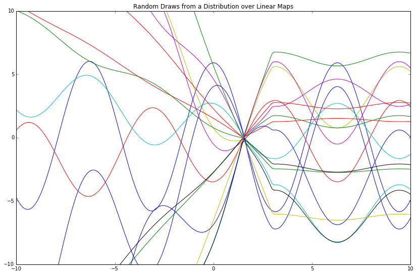
This distribution over linear maps gives a distribution over functions, where the "mean function" is $\phi(X)^T\mu_w$ (which reads directly from the mu_lm variable above).

Notwithstanding, I find this phrasing to be confusing; to me, a "distribution over functions" sounds like some opaque object that spits out algebraic symbols via logic miles above my cognitive ceiling. As such, I instead think of this in more intuitive terms as a distribution over function evaluations, where a single function evaluation is a list of (x, y) tuples and nothing more.

For example, given a vector x = np.array([1, 2, 3]) and a function lambda x: x**2, an evaluation of this function gives y = np.array([1, 4, 9]). We now have tuples [(1, 1), (2, 4), (3, 9)] from which we can create a line plot. This gives one "function evaluation."

Above, we sampled 17 function evaluations, then plotted the 200 resulting (x, y) tuples (as our input was a 200D vector $X$) for each. The evaluations are similar because of the given mean function mu_lm; they are different because of the given covariance matrix cov_lm.

Let's try some different "features" for our x-values then plot the same thing.

# Make different, though still arbitrary, features
phi_x = np.array([x ** (1 + i) for i in range(2)])

png

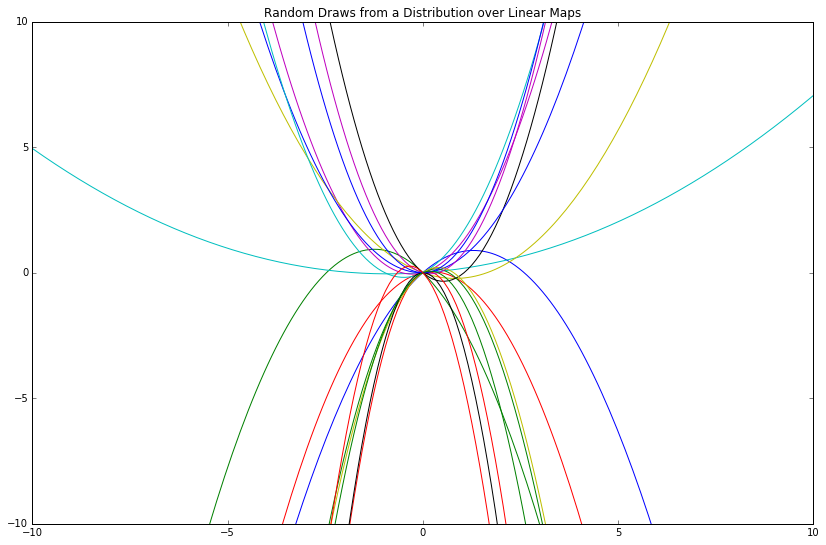
"The features we choose give a 'language' with which we can express a relationship between $x$ and $y$."¹ Some features are more expressive than others; some restrict us entirely from expressing certain relationships.

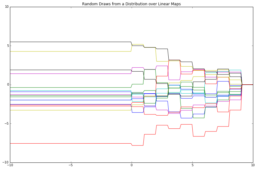
For further illustration, let's employ step functions as features and see what happens.

# Make features, as before
phi_x = np.array([x < i for i in range(10)])

png

Gaussians are closed under conditioning and marginalization

Let's revisit the 2D Gaussians plotted above. They took the form

$$ (x, y) \sim \mathcal{N}(\mu, \Sigma) $$

where $\mathcal{N}$ denotes the Normal, i.e. Gaussian distribution.

Said differently:

$$ P(x, y) = \mathcal{N}(\mu, \Sigma) $$

And now a bit more rigorously:

$$ P(x, y) = \mathcal{N}\bigg([\mu_x, \mu_y], \begin{bmatrix} \Sigma_x & \Sigma_{xy}\\ \Sigma_{xy}^T & \Sigma_y\\ \end{bmatrix}\bigg) $$

NB: In this case, all 4 "Sigmas" in the 2x2 covariance matrix are floats. If our covariance were bigger, say 31x31, then these 4 Sigmas would be matrices (with an aggregate size totaling 31x31).

What if we wanted to know the distribution over $y$ conditional on $x$ taking on a certain value, e.g. $P(y\vert x > 1)$?

$y$ is a single element, so the resulting conditional will be a univariate distribution. To gain intuition, let's do this in a very crude manner:

y_values = []
mu, cov = np.array([0, 0]), np.diag([1, 1])
while len(y_values) < 345:  # some random sample size
    x, y = np.random.multivariate_normal(mu, cov)
    if x > 1:
        y_values.append(y)

plt.figure(figsize=(8, 5))
pd.Series(y_values).hist(grid=False, bins=15)
_ = plt.title('Histogram of y-values, when x > 1')

png

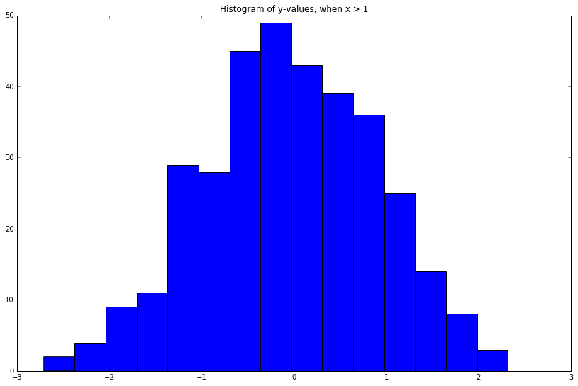
Cool! Looks kind of Gaussian as well.

Instead, what if we wanted to know the functional form of the real density, $P(y\vert x)$, instead of this empirical distribution of its samples? One of the axioms of conditional probability tells us that:

$$ P(y\vert x) = \frac{P(x, y)}{P(x)} = \frac{P(x, y)}{\int P(x, y)dy} $$

The right-most denominator can be written as:

$$ \begin{align*} \int P(x, y)dy &= \int \mathcal{N}\bigg([\mu_x, \mu_y], \begin{bmatrix} \Sigma_x & \Sigma_{xy}\\ \Sigma_{xy}^T & \Sigma_y\\ \end{bmatrix}\bigg) dy\\ \\ &= \mathcal{N}(\mu_x, \Sigma_x) \end{align*} $$

Marginalizing a > 1D Gaussian over one of its elements yields another Gaussian: you just "pluck out" the elements you'd like to examine. In other words, Gaussians are closed under marginalization. "It's almost too easy to warrant a formula."¹

As an example, imagine we had the following Gaussian $P(a, b, c)$, and wanted to compute the marginal over the first 2 elements, i.e. $P(a, b) = \int P(a, b, c)dc$:

# P(a, b, c)
mu = np.array([3, 5, 9])
cov = np.array([
    [11, 22, 33],
    [44, 55, 66],
    [77, 88, 99]
])

# P(a, b)
mu_marginal = np.array([3, 5])
cov_marginal = np.array([
    [11, 22],
    [44, 55]
])

# That's it.

Finally, we compute the conditional Gaussian of interest—a result well-documented by mathematicians long ago:

$$ \begin{align*} P(y\vert x) &= \frac{ \mathcal{N}\bigg( [\mu_x, \mu_y], \begin{bmatrix} \Sigma_x & \Sigma_{xy}\\ \Sigma_{xy}^T & \Sigma_y\\ \end{bmatrix} \bigg) } {\mathcal{N}(\mu_x, \Sigma_x)}\\ \\ &= \mathcal{N}(\mu_y + \Sigma_{xy}\Sigma_x^{-1}(x - \mu_x), \Sigma_y - \Sigma_{xy}\Sigma_x^{-1}\Sigma_{xy}^T) \end{align*} $$

$x$ can be a matrix. From there, just plug stuff in.

Conditioning a > 1D Gaussian on one (or more) of its elements yields another Gaussian. In other words, Gaussians are closed under conditioning.

Inferring the weights

We previously posited a distribution over some vector of weights, $w \sim \text{Normal}(\mu_w, \Sigma_w)$. In addition, we posited a distribution over the linear map of these weights onto some matrix $A = \phi(X)^T$:

$$ y = \phi(X)^Tw \sim \text{Normal}(\phi(X)^T\mu_w,\ \phi(X)^T\Sigma_w \phi(X)) $$

Given some ground-truth samples from this distribution $y = \phi(X)^Tw$, i.e. ground-truth "function evaluations," we'd like to infer the weights $w$ most consistent with $y$.

In machine learning, we equivalently say that given a model and some observed data (X_train, y_train), we'd like to compute/train/optimize the weights of said model.

Most precisely, our goal is to infer $P(w\vert y)$ (where $y$ are our observed function evaluations). To do this, we simply posit a joint distribution over both quantities:

$$ P(w, y) = \mathcal{N}\bigg( [\mu_w, \phi(X)^T\mu_w], \begin{bmatrix} \Sigma_w & \Sigma_{wy}\\ \Sigma_{wy}^T & \phi(X)^T\Sigma_w \phi(X)\\ \end{bmatrix} \bigg) $$

Then compute the conditional via the formula above:

$$ \begin{align*} P(w\vert y) &= \mathcal{N}(\mu_w + \Sigma_{wy}\Sigma_y^{-1}(y - \mu_y), \Sigma_w - \Sigma_{wy}\Sigma_y^{-1}\Sigma_{wy}^T)\\ \\ &= \mathcal{N}(\mu_w + \Sigma_{wy}(\phi(X)^T\Sigma_w \phi(X))^{-1}(y - \mu_w^T \phi(X)), \Sigma_w - \Sigma_{wy}(\phi(X)^T\Sigma_w \phi(X))^{-1}\Sigma_{wy}^T) \end{align*} $$

This formula gives the posterior distribution over our weights $P(w\vert y)$ given the model and observed data tuples (x, y).

Until now, we've assumed a 2D $w$, and therefore a $\phi(X)$ in $\mathbb{R}^2$ as well. Moving forward, we'll work with weights and features in a higher-dimensional space, $\mathbb{R}^{20}$; this will give us a more expressive language with which to capture the true relationship between some quantity $x$ and its corresponding $y$. $\mathbb{R}^{20}$ is an arbitrary choice; it could have been $\mathbb{R}^{17}$, or $\mathbb{R}^{31}$, or $\mathbb{R}^{500}$ as well.

# The true function that maps `x` to `y`. This is what we are trying to recover with our mathematical model.
def true_function(x):
    return np.sin(x)**2 - np.abs(x - 3) + 7


# x-values
x_train = np.array([-5, -2.5, -1, 2, 4, 6])


# y-train
y_train = true_function(x_train)


# Params of distribution over weights
D = 20
mu_w = np.zeros(D)  # mu_w.shape: (D,)
cov_w = 1.1 * np.diag(np.ones(D))  # cov_w.shape: (D, D)


# A function to make some arbitrary features
def phi_func(x):
    return np.array([np.abs(x - d) for d in range(int(-D / 2), int(D / 2))])  # phi_x.shape(D, len(x))


# A function that computes the parameters of the linear map distribution
def compute_linear_map_params(mu, cov, map_matrix):
    mu_lm = map_matrix.T @ mu
    cov_lm = map_matrix.T @ cov @ map_matrix
    return mu_lm, cov_lm


def compute_weights_posterior(mu_w, cov_w, phi_func, x_train, y_train):
    """
    NB: "Computing a posterior," and given that that posterior is Gaussian, implies nothing more than
    computing the mean-vector and covariance matrix of this Gaussian.
    """
    # Featurize x_train
    phi_x = phi_func(x_train)

    # Params of prior distribution over function evals
    mu_y, cov_y = compute_linear_map_params(mu_w, cov_w, phi_x)

    # Params of posterior distribution over weights
    mu_w_post = mu_w + cov_w @ phi_x @ np.linalg.inv(cov_y) @ (y_train - mu_y)
    cov_w_post = cov_w - cov_w @ phi_x @ np.linalg.inv(cov_y) @ phi_x.T @ cov_w

    return mu_w_post, cov_w_post


# Compute weights posterior
mu_w_post, cov_w_post = compute_weights_posterior(mu_w, cov_w, phi_func, x_train, y_train)

As with our prior over our weights, we can equivalently draw samples from the posterior over our weights, then plot. These samples will be 20D vectors; we reduce them to 2D for ease of visualization.

# Draw samples
samples_prior = np.random.multivariate_normal(mu_w, cov_w, size=250)
samples_post = np.random.multivariate_normal(mu_w_post, cov_w_post, size=250)

# Reduce to 2D for ease of visualization
first_dim_prior, second_dim_prior = zip(*TSNE(n_components=2).fit_transform(samples_prior))
first_dim_post, second_dim_post = zip(*TSNE(n_components=2).fit_transform(samples_post))

png

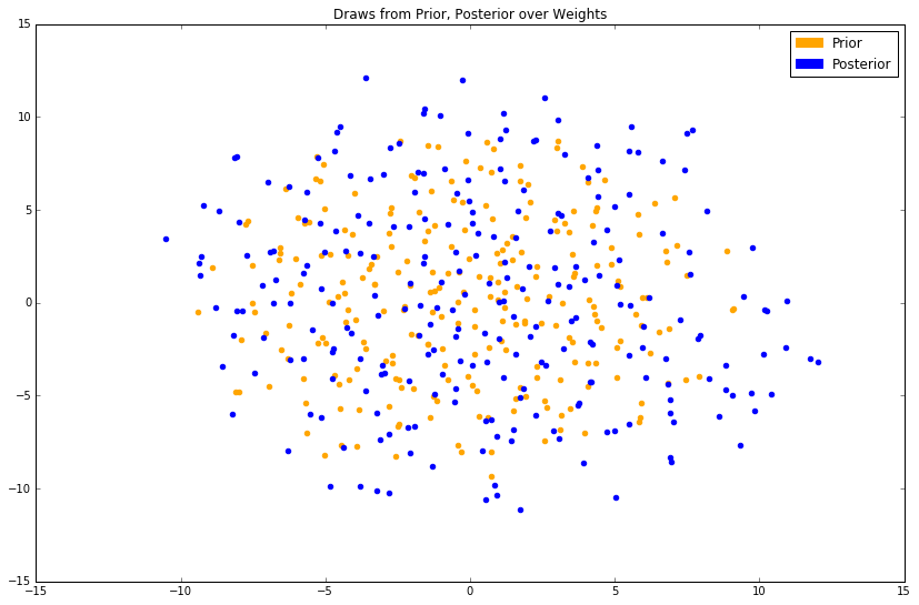
Samples from the prior are plotted in orange; samples from the posterior are plotted in blue. As this is a stochastic dimensionality-reduction algorithm, the results will be slightly different each time.

At best, we can see that the posterior has slightly larger values in its covariance matrix, evidenced by the fact that the blue cloud is more disperse than the orange, and has probably maintained a similar mean. The magnitude of change (read: a small one) is expected, as we've only conditioned on 6 ground-truth tuples.

Predicting on new data

Previously, we sampled function evaluations by centering a multivariate Gaussian on $\phi(X)^T\mu_{w}$, where $\mu_w$ was the mean of the prior distribution over weights. We'd now like to do the same thing, but use our posterior over weights instead. How does this work?

Well, Gaussians are closed under linear maps. So, we just follow the formula we had used above.

This time, instead of input vector $X$, we'll use a new input vector called $X_{*}$, i.e. the "new data" on which we'd like to predict.

$$ \phi(X_{*})^Tw \sim \text{Normal}(\phi(X_{*})^T\mu_{w, \text{post}},\ \phi(X_{*})^T \Sigma_{w, \text{post}}\phi(X_{*})) $$

This gives us a posterior distribution over function evaluations.

In machine learning parlance, this is akin to: given some test data X_test, and a model whose weights were trained/optimized with respect to/conditioned on some observed ground-truth tuples (X_train, y_train), we'd like to generate predictions y_test, i.e. samples from the posterior over function evaluations.

The function to compute this posterior, i.e. compute the mean-vector and covariance matrix of this Gaussian, will appear both short and familiar.

x_test = np.linspace(-10, 10, 200)


def compute_gp_posterior(mu_w, cov_w, phi_func, x_train, y_train, x_test):
    mu_w_post, cov_w_post = compute_weights_posterior(mu_w, cov_w, phi_func, x_train, y_train)
    phi_x_test = phi_func(x_test)
    mu_y_post, cov_y_post = compute_linear_map_params(mu_w_post, cov_w_post, phi_x_test)
    return mu_y_post, cov_y_post


mu_y_post, cov_y_post = compute_gp_posterior(mu_w, cov_w, phi_func, x_train, y_train, x_test)

To plot, we typically just plot the error bars, i.e. the space within (mu_y_post - var_y_post, mu_y_post + var_y_post) for each x, as well as the ground-truth tuples as big red dots. This gives nothing more than a picture of the mean-vector and covariance of our posterior. Optionally, we can plot samples from this posterior as well, as we did with our prior.

def plot_gp_posterior(mu_y_post, cov_y_post, x_train, y_train, x_test, n_samples=0, ylim=(-3, 10)):
    plt.figure(figsize=(14, 9))
    plt.ylim(*ylim)
    plt.xlim(-10, 10)
    plt.title('Posterior Distribution over Function Evaluations')

    # Extract the variances, i.e. the diagonal, of our covariance matrix
    var_y_post = np.diag(cov_y_post)

    # Plot the error bars.
    # To do this, we fill the space between `(mu_y_post - var_y_post, mu_y_post + var_y_post)` for each `x`
    plt.fill_between(x_test, mu_y_post - var_y_post, mu_y_post + var_y_post, color='#23AEDB', alpha=.5)

    # Scatter-plot our original 6 `(x, y)` tuples
    plt.plot(x_train, y_train, 'ro', markersize=10)

    # Optionally plot actual samples (function evaluations) from this posterior
    if n_samples > 0:
        for _ in range(n_samples):
            y_pred = np.random.multivariate_normal(mu_y_post, cov_y_post)
            plt.plot(x_test, y_pred, alpha=.2)


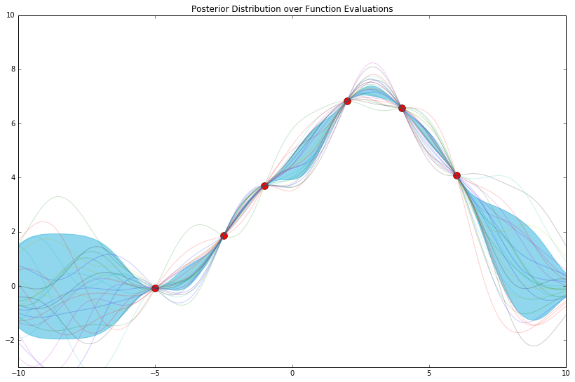
plot_gp_posterior(mu_y_post, cov_y_post, x_train, y_train, x_test, n_samples=25)

png

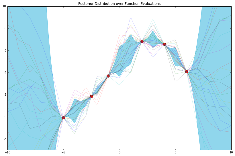
The posterior distribution is nothing more than a distribution over function evaluations (from which we've sampled 25 function evaluations above) most consistent with our model and observed data tuples. As such, and to give further intuition, a crude way of computing this distribution might be continuously drawing samples from our prior over function evaluations, and keeping only the ones that pass through, i.e. are "most consistent with," all of the red points above.

Finally, we stated before that the features we choose (i.e. our phi_func) give a "language" with which we can express the relationship between $x$ and $y$. Here, we've chosen a language with 20 words. What if we chose a different 20?

D = 20


# Params of distribution over weights
mu_w = np.zeros(D)  # mu_w.shape: (D,)
cov_w = 1.1 * np.diag(np.ones(D))  # cov_w.shape: (D, D)


# Still arbitrary, i.e. a modeling choice!
def phi_func(x, D=D, a=.25):
    return np.array([a * np.cos(i * x) for i in range(int(-D / 2), int(D / 2))])  # phi_x.shape: (D, len(x))


mu_y_post, cov_y_post = compute_gp_posterior(mu_w, cov_w, phi_func, x_train, y_train, x_test)
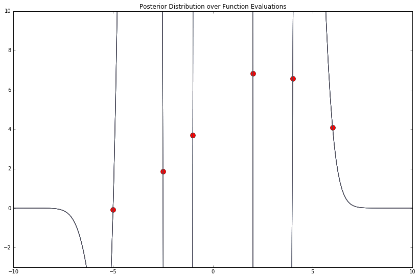
plot_gp_posterior(mu_y_post, cov_y_post, x_train, y_train, x_test, n_samples=25)

png

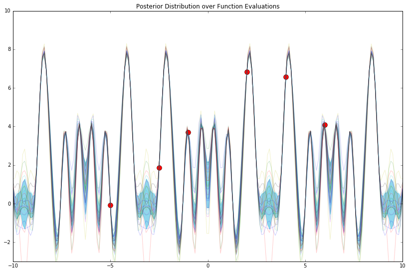
Not great. As a brief aside, how do we read the plot above? It's simply a function, a transformation, a lookup: given an $x$, it tells us the corresponding expected value $y$, and the variance around this estimate.

For instance, right around $x = -3$, we can see that $y$ is somewhere in $[-1, 1]$; given that we've only conditioned on 6 "training points," we're still quite unsure as to what the true answer is. To this effect, a GP (and other fully-Bayesian models) allows us to quantify this uncertainty judiciously.

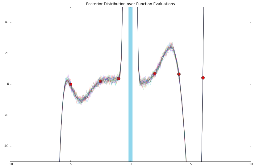
Now, let's try some more features and examine the model we're able to build.

# Still arbitrary, i.e. a modeling choice!
def phi_func(x, D=D, a=1e-5):
    return np.array([a * (x ** i) for i in range(int(-D / 2), int(D / 2))])  # phi_x.shape: (D, len(x))

png

def phi_func(x, D=D):
    return np.array([np.exp(-.5 * (x - d)**2) for d in range(int(-D / 2), int(D / 2))])  # phi_x.shape: (D, len(x))

png

That last one might look familiar. Therein, the features we chose (still arbitrarily, really) are called "radial basis functions" (among other names).

We've loosely examined what happens when we change the language through which we articulate our model. Next, what if we changed the size of its vocabulary?

First, let's backtrack, and try 8 of these radial basis functions instead of 20.

D = 8


# Params of distribution over weights
mu_w = np.zeros(D)  # mu_w.shape: (D,)
cov_w = 1.1 * np.diag(np.ones(D))  # cov_w.shape: (D, D)


def phi_func(x, D=D):
    return np.array([np.exp(-.5 * (x - d)**2) for d in range(int(-D / 2), int(D / 2))])  # phi_x.shape: (D, len(x))


mu_y_post, cov_y_post = compute_gp_posterior(mu_w, cov_w, phi_func, x_train, y_train, x_test)
plot_gp_posterior(mu_y_post, cov_y_post, x_train, y_train, x_test, n_samples=25)

png

Very different! Holy overfit. What about 250?

D = 250


# Params of distribution over weights
mu_w = np.zeros(D)  # mu_w.shape: (D,)
cov_w = 1.1 * np.diag(np.ones(D))  # cov_w.shape: (D, D)


def phi_func(x, D=D):
    return np.array([np.exp(-.5 * (x - d)**2) for d in range(int(-D / 2), int(D / 2))])  # phi_x.shape: (D, len(x))


mu_y_post, cov_y_post = compute_gp_posterior(mu_w, cov_w, phi_func, x_train, y_train, x_test)
plot_gp_posterior(mu_y_post, cov_y_post, x_train, y_train, x_test, n_samples=25)

png

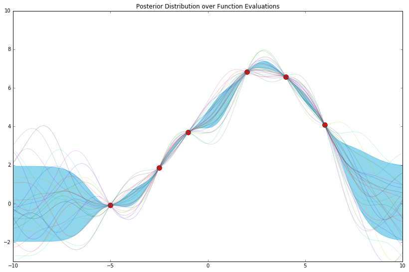
It appears that the more features we use, the more expressive, and/or less endemically prone to overfitting, our model becomes.

So, how far do we take this? D = 1000? D = 50000? How high can we go? We'll pick up here in the next post.

Summary

In this tutorial, we've arrived at the mechanical notion of a Gaussian process via simple Gaussian algebra.

Thus far, we've elucidated the following ideas:

A Gaussian process (GP) defines a distribution over functions (i.e. function evaluations) ✅
Marginalizing a Gaussian over a subset of its elements gives another Gaussian (just pluck out the pieces of interest) ✅
Conditioning a subset of the elements of a Gaussian on another subset gives another Gaussian (a simple algebraic formula) ✅
Posterior over functions (the linear map of the posterior over weights onto some matrix $A = \phi(X_{*})^T$) ✅
Covariances (the second thing we need in order to specify a multivariate Gaussian) ✅

Conversely, we did not yet cover (directly):

Kernels
Squared-exponentials
"A Gaussian process is non-parametric, i.e. it has an infinite number of parameters"

These will be the subject of the following post. Thanks for reading.

Code

The repository and rendered notebook for this project can be found at their respective links.

References

Gaussian Processes 1 - Philipp Hennig - MLSS 2013 Tübingen (from which this post takes heavy inspiration) ↩↩
Gaussian Processes for Machine Learning. Carl Edward Rasmussen and Christopher K. I. Williams The MIT Press, 2006. ISBN 0-262-18253-X. ↩
Fitting Gaussian Process Models in Python ↩
Gaussian process regression ↩

From Gaussian Algebra to Gaussian Processes, Part 1

Will Wolf