Abstract
Implicit Matrix Factorization
The Implicit Matrix Factorization (IMF) algorithm as presented by Hu, Koren and Volinksy is a widely popular, effective method for recommending items to users. This approach was born from necessity: while explicit feedback as to our users' tastes - a questionnaire completed at user signup, for example - makes building a recommendation engine straightforward, we often have nothing more than implicit feedback data - view count, click count, time spent on page, for example - which serve instead as a proxy for these preferences. Crucially, the latter feedback is asymmetric: while a high view count might indicate positive preference for a given item, a low view count cannot be said to do the opposite. Perhaps, the user simply didn't know the item was there.
IMF begins with a ratings matrix $R$, where $R_{u, i}$ gives the implicit feedback value observed for user $u$ and item $i$. Next, it constructs two other matrices defined as follows:
$$ p_{u, i} = \begin{cases} 1 & r_{u, i} \gt 0\\ 0 & r_{u, i} = 0 \end{cases}\\ c_{u, i} = 1 + \alpha r_{u, i} $$$P$ gives a binary matrix indicating our belief in the existence of each user's preference for each item. $C$ gives our confidence in the existence of each user's preference for each item where, trivially, larger values of $r_{u, i}$ give us higher confidence that user $u$ indeed likes item $i$.
Next, IMF outlines its goal: let's embed each user and item into $\mathbb{R}^f$ such that their dot product approximates the former's true preference for the latter. Finally, and naming user vectors $x_u \in \mathbb{R}^f$ and item vectors $y_i \in \mathbb{R}^f$, we compute the argmin of the following objective:
$$ \underset{x_{*}, y_{*}}{\arg\min}\sum\limits_{u, i}c_{u, i}\big(p_{u, i} - x_u^Ty_i\big)^2 + \lambda\bigg(\sum\limits_u\|x_u\|^2 + \sum\limits_i\|y_u\|^2\bigg) $$Once sufficiently minimized, we can compute expected preferences $\hat{p}_{u, i} = x_u^Ty_i$ for unobserved $\text{(user, item)}$ pairs; recommendation then becomes:
- For a given user $u$, compute predicted preferences $\hat{p}_{u, i} = x_u^Ty_i$ for all items $i$.
- Sort the list in descending order.
- Returning the top $n$ items.
Shallow neural networks
IMF effectively gives a function $f: u, i \rightarrow \hat{p}_{u, i}$. As before, our goal is to minimize the function above, which we can now rewrite as:
$$ \underset{x_{*}, y_{*}}{\arg\min}\sum\limits_{u, i}c_{u, i}\big(p_{u, i} - f(u, i)\big)^2 + \lambda\bigg(\sum\limits_u\|x_u\|^2 + \sum\limits_i\|y_u\|^2\bigg) $$To approximate this function, I turn to our favorite universal function approximator: neural networks optimized with stochastic gradient descent.
This work is built around a toy web application I authored long ago: dotify. At present, dotify:
- Pulls data nightly from Spotify Charts. These data contain the number of streams for that day's top 200 songs for each of 55 countries.
- Computes an implicit matrix factorization nightly, giving vectors for both countries and songs.
- Allows the user to input a "country-arithmetic" expression, i.e. "I want music like
Colombia x Turkey - Germany." It then performs this arithmetic with the chosen vectors and recommends songs to the composite.
In this work, I first fit and cross-validate an implicit matrix factorization model, establishing the three requisite parameters: $f$, the dimensionality of the latent vectors; $\alpha$, the scalar multiple used in computing $C$; $\lambda$ the regularization strength used in on our loss function.
Network architectures
Next, I explore five different shallow neural network architectures in attempt to improve upon the observed results. These architectures are as follows:
- A trivially "Siamese" network which first embeds each country and song index into $\mathbb{R}^f$ in parallel then computes a dot-product of the embeddings. This is roughly equivalent to what is being done by IMF.
- Same as previous, but with a bias embedding for each set, in $\mathbb{R}$, added to the dot-product.
- Same as #1, but concatenate the vectors instead. Then, stack 3 fully-connected layers with ReLU activations, batch normalization after each, and dropout after the first. Finally, add a 1-unit dense layer on the end, and add bias embeddings to the result. (NB: I wanted to add the bias embeddings to the respective $\mathbb{R}^f$ embeddings at the outset, but couldn't figure out how to do this in Keras.)
- Same as #2, except feed in the song title text as well. This text is first tokenized, then padded to a maximum sequence length, then embedded into a fixed-length vector by an LSTM, then reduced to a single value by a dense layer with a ReLU activation. Finally, this scalar is concatenated to the scalar output that #2 would produce, and the result is fed into a final dense layer with a linear activation - i.e. a linear combination of the two.
- Same as #4, except feed in the song artist index as well. This index is first embedded into a vector, then reduced to a scalar by a dense layer with a ReLU activation. Finally, this scalar is concatenated with the two scalars produced in the second-to-last layer of #4, then fed into a final dense layer with a linear activation. Like the previous, this is a linear combination of the three inputs.
Results
While the various network architectures are intruiging for both the ease with which we can incorporate multiple, disparate inputs into our function, and the ability to then train this function end-to-end with respect to our main minimization objective, we find no reason to prefer them over the time-worn Implicit Matrix Factorization algorithm.
Data preparation
To construct our ratings matrix, I take the sum of total streams for each $\text{(country, song)}$ pair. The data are limited to a given number of "top songs," defined as a song that appeared on Spotify Charts on a given date.
Because the values exist on wildly different orders of magnitude, I scale the results as follows:
$$\tilde{r}_{u, i} = \log{\bigg(\frac{1 + r_{u, i}}{\epsilon}\bigg)}$$To start, let's build a ratings matrix for a small sample of the data.
ratings_matrix = RatingsMatrix(n_top_songs=10000, eps=1e3)
ratings_matrix.R_ui.head()
Next, let's get an idea of the sparsity of our data and how many songs each country has streamed.
sparsity = (ratings_matrix.R_ui == 0).mean().mean()
non_zero_entries_percent = 100*np.round(1 - sparsity, 4)

print('Our ratings matrix has {}% non-zero entries.'.format(non_zero_entries_percent))
print('Our ratings matrix contains {} countries and {} unique songs.'.format(*ratings_matrix.R_ui.shape))
plt.figure(figsize=(10, 6))

songs_rated_by_country = (ratings_matrix.R_ui > 0).sum(axis=1)
plt.hist(songs_rated_by_country)
plt.title('Distribution of # of Unique Songs Streamed per Country', fontsize=15)
plt.xlabel('Unique Songs Streamed', fontsize=12)
_ = plt.ylabel('# of Countries', fontsize=12)

Construct training, validation sets
In reviewing literature on recommender engine evaluation, it seems common to create training and validation sets as follows:
- Filter your ratings matrix for users (countries) that meet some criterion, i.e. they've streamed above a certain threshold of songs.
- Select a random $x\%$ of their items (songs).
- "Move" these items into a validation matrix; set them to 0 in the training matrix.
To construct this split, I first compute a sensible threshold for Step #1, then "move" a random 20% of songs from the training matrix to the validation matrix.
print('The 15th percentile of songs rated by country is {}.'.format(
    np.percentile(songs_rated_by_country, 15)
))
Let's choose 50 songs as our cutoff, and move 20% of the songs in qualifying rows to a validation set.
NB: The actual ratings matrix is located at RatingsMatrix.R_ui. This reflects an API choice I made when first starting this project.
def split_ratings_matrix_into_training_and_validation(ratings_matrix, eligibility_mask, fraction_to_drop=.2):
    training_matrix = ratings_matrix
    validation_matrix = deepcopy(training_matrix)
    validation_matrix.R_ui = pd.DataFrame(0., index=training_matrix.R_ui.index, columns=training_matrix.R_ui.columns)

    for country_id, ratings in training_matrix.R_ui[eligibility_mask].iterrows():

        rated_songs_mask = training_matrix.R_ui.ix[country_id] > 0
        rated_songs = training_matrix.R_ui.ix[country_id][rated_songs_mask].index.tolist()
        n_songs_to_drop = int( len(rated_songs)*fraction_to_drop )
        songs_to_drop = set( random.sample(rated_songs, n_songs_to_drop) )

        validation_matrix.R_ui.ix[country_id][songs_to_drop] = training_matrix.R_ui.ix[country_id][songs_to_drop]
        training_matrix.R_ui.ix[country_id][songs_to_drop] = 0.

    return training_matrix, validation_matrix
more_than_50_ratings_mask = songs_rated_by_country > 50

training_matrix, validation_matrix = split_ratings_matrix_into_training_and_validation(
    ratings_matrix=ratings_matrix,
    eligibility_mask=more_than_50_ratings_mask
)
Evaluation
Evaluating recommender systems is an inexact science because there is no "right" answer. In production, this evaluation is often done via the A/B test of a proxy metric important to the business - revenue, for example. In training, the process is less clear. To this end, the authors of the IMF paper offer the following:
Evaluation of implicit-feedback recommender requires appropriate measures. In the traditional setting where a user is specifying a numeric score, there are clear metrics such as mean squared error to measure success in prediction. However with implicit models we have to take into account availability of the item, competition for the item with other items, and repeat feedback. For example, if we gather data on television viewing, it is unclear how to evaluate a show that has been watched more than once, or how to compare two shows that are on at the same time, and hence cannot both be watched by the user.
Additionally, they state:
It is important to realize that we do not have a reliable feedback regarding which programs are unloved, as not watching a program can stem from multiple different reasons. In addition, we are currently unable to track user reactions to our recommendations. Thus, precision based metrics are not very appropriate, as they require knowing which programs are undesired to a user. However, watching a program is an indication of liking it, making recall-oriented measures applicable.
In solution, they propose evaluating the "expected percentile ranking" defined as follows:
$$ \overline{\text{rank}} = \frac{\sum_{u, i}\tilde{r}_{u, i}^t\text{rank}_{u, i}}{\sum_{u, i}\tilde{r}_{u, i}^t} $$Here, $\text{rank}_{u, i}$ gives the percentile-ranking of the predicted preference, i.e. if $\hat{p}_{u = 17, i = 34}$ is the largest of all predicted preferences, then $\text{rank}_{u = 17, i = 34} = 0\%$. Similarly, the smallest of the predicted preferences, i.e. the last on the list, equals $100\%$.
The following class accepts a training matrix, validation matrix and a matrix of predicted preferences. It then exposes the mean expected percentile ranking for both training and validation sets as properties on the instance.
class ExpectedPercentileRankingsEvaluator:

    def __init__(self, training_matrix, validation_matrix, eligibility_mask, predicted_preferences):
        self.training_matrix = training_matrix
        self.validation_matrix = validation_matrix
        self.eligibility_mask = eligibility_mask
        self.predicted_preferences = predicted_preferences
        self._expected_percentile_rankings_train = []
        self._expected_percentile_rankings_validation = []

    def run(self):
        self._evaluate_train()
        self._evaluate_validation()

    def _evaluate_train(self):
        self._expected_percentile_rankings_train = self._evaluate(matrix=self.training_matrix)

    def _evaluate_validation(self):
        self._expected_percentile_rankings_validation = self._evaluate(matrix=self.validation_matrix)

    def _evaluate(self, matrix):
        expected_percentile_rankings = []
        for country_id, preferences in self.predicted_preferences[self.eligibility_mask].iterrows():
            predictions = pd.DataFrame({
                'predicted_preference': preferences.sort_values(ascending=False),
                'rank': np.arange( len(preferences) ),
                'percentile_rank': np.arange( len(preferences) ) / len(preferences)
            })
            ground_truth = matrix.R_ui.ix[country_id][ matrix.R_ui.ix[country_id] > 0 ]
            numerator = (ground_truth * predictions['percentile_rank'][ground_truth.index]).sum()
            denominator = ground_truth.sum()
            expected_percentile_rankings.append( numerator / denominator )

        return expected_percentile_rankings

    @property
    def mean_expected_percentile_rankings_train(self):
        return np.mean(self._expected_percentile_rankings_train)

    @property
    def mean_expected_percentile_rankings_validation(self):
        return np.mean(self._expected_percentile_rankings_validation)
Grid search
Next, we perform a basic grid search to find reasonable values for $\alpha$ and $\lambda$.
F = 30
grid_search_results = {}
result = namedtuple('Result', 'alpha lmbda')
alpha_values = [1e-1, 1e0, 1e1, 1e2]
lmbda_values = [1e-1, 1e0, 1e1, 1e2]

for alpha in alpha_values:
    for lmbda in lmbda_values:
        implicit_mf = ImplicitMF(ratings_matrix=training_matrix, f=F, alpha=alpha, lmbda=lmbda)
        implicit_mf.run()
        predicted_preferences = implicit_mf.country_vectors.vectors.dot( implicit_mf.song_vectors.vectors.T )

        evaluator = ExpectedPercentileRankingsEvaluator(
            training_matrix=training_matrix,
            validation_matrix=validation_matrix,
            eligibility_mask=more_than_50_ratings_mask,
            predicted_preferences=predicted_preferences
        )
        evaluator.run()
        grid_search_results[result(alpha=alpha, lmbda=lmbda)] = {
            'train': evaluator.mean_expected_percentile_rankings_train,
            'validation': evaluator.mean_expected_percentile_rankings_validation
        }
        print(grid_search_results)
Let's visualize the results for clarity. I plot the opposite of the validation score such that the parameters corresponding to the darkest square are most favorable.
grid_search_items = [(params, results) for params, results in grid_search_results.items()]
grid_search_items.sort(key=lambda tup: tup[0].alpha)

params, results = zip(*grid_search_items)
validation_results = np.array([result['validation'] for result in results]).reshape(4, 4)

plt.figure(figsize=(15, 10))
plt.xticks([])
plt.yticks([])
plt.pcolormesh(-validation_results, cmap='Reds')
plt.colorbar()
for alpha_index, alpha in enumerate(alpha_values):
    for lbmda_index, lmbda in enumerate(lmbda_values):
        plt.text(
            x = lbmda_index + 0.5,
            y = alpha_index + 0.5,
            s = r'$\alpha$ = {}'.format(alpha) + '\n' + r'$\lambda$ = {}'.format(lmbda),
            ha='center',
            va='center',
            size=15,
            color='w'
        )
plt.title('Grid Search Results', fontsize=15)
plt.xlabel(r'$\lambda$ Values', fontsize=14)
_ = plt.ylabel(r'$\alpha$ Values', fontsize=14)

best_params = min(grid_search_results, key=lambda key: grid_search_results.get(key)['validation'])
print('The best parameters were found to be: {}.'.format(best_params))
Train a final model
Using these parameters, let's train a final implicit matrix factorization model using 1,000,000 top songs. Additionally, we'll choose $\epsilon = 1,000$ which seemed to work best in simple experimentation. This experimentation is not shown here.
ratings_matrix = RatingsMatrix(n_top_songs=1000000, eps=1e3)
print('Our ratings matrix contains {} countries and {} unique songs.'.format(*ratings_matrix.R_ui.shape))
implicit_mf = ImplicitMF(ratings_matrix=ratings_matrix, f=F, alpha=best_params.alpha, lmbda=best_params.lmbda)
implicit_mf.run()
Visualize
Let's plot the cosine similarities between all pairs of countries to confirm that things make sense. Intuitively, I'd think that countries in the following groups should be similar:
- United States, United Kingdom, Canada, Australia, New Zealand
- Latin American countries
- Sweden, Finland, Norway, Denmark
First let's replace the index of our vectors such that it contains the country names.
country_vectors_df = implicit_mf.country_vectors.vectors.copy()

country_id_to_name = {countries_lookup[name]['id']: name for name in countries_lookup}
country_ids = country_vectors_df.index
country_names = pd.Index([country_id_to_name[c_id] for c_id in country_ids], name='country_name')
country_vectors_df.index = country_names

country_vectors_df.head()
Then, we'll plot the cosine similarities.
sns.set(style="white")

def plot_cosine_similarities(country_vectors_df):

    similarities_df = pd.DataFrame(
        data=cosine_similarity(country_vectors_df),
        index=country_vectors_df.index,
        columns=country_vectors_df.index
    )

    lower_triangle_mask = np.zeros_like(similarities_df, dtype=np.bool)
    lower_triangle_mask[np.triu_indices_from(lower_triangle_mask)] = True

    f, ax = plt.subplots(figsize=(21, 21))
    cmap = sns.diverging_palette(220, 10, as_cmap=True)

    sns.heatmap(
        similarities_df,
        mask=lower_triangle_mask,
        cmap=cmap,
        vmax=.5,
        square=True,
        xticklabels=True,
        yticklabels=True,
        linewidths=1,
        cbar_kws={"shrink": .5},
        ax=ax,
    )
    ax.set_title('Cosine Similarity Matrix', fontsize=20)
plot_cosine_similarities(country_vectors_df)

I first turn to my favorite country - Colombia - to inspect its similarity with other Latin American countries. The numbers are high for: Peru, Paraguay, Panama, Nicaragua, Gautemala, Ecuador, Dominican Republic and Costa Rica.
Next, I turn to the United Kingdom: it is most similar with Switzerland, New Zealand, Ireland, Hungary, Belgium and Australia.
Finally, we see that Sweden is similar enough to Norway, yet not Finland (who, incidentally, seems to have nothing in common with anyone at all).
Overall, this looks very good to me.
Visualize with TSNE
To further inspect similarities between countries, let's explore the 2-dimensional TSNE space.
tsne = TSNE(perplexity=30, n_components=2, init='pca', n_iter=5000, random_state=12345)

country_embeddings = pd.DataFrame(
    data=tsne.fit_transform(country_vectors_df),
    index=country_vectors_df.index,
    columns=['dim_1', 'dim_2']
)
def plot_tsne_embeddings(country_embeddings):

    plt.figure(figsize=(15,15))

    for country_name, country_embedding in country_embeddings.iterrows():
        dim_1, dim_2 = country_embedding
        plt.scatter(dim_1, dim_2)
        plt.annotate(country_name, xy=(dim_1, dim_2), xytext=(5, 2), textcoords='offset points', ha='right', va='bottom')
        plt.title('Two-Dimensional TSNE Embeddings of Latent Country Vectors', fontsize=16)
        plt.xlabel('Dimension 1', fontsize=12)
        plt.ylabel('Dimension 2', fontsize=12)
    plt.show()
plot_tsne_embeddings(country_embeddings)

This is not particularly useful. Furthermore, and perhaps most importantly, the plot varies immensely when changing the random seed. This is a worthwhile step nonetheless.
Inspect predicted preferences
Crucially, we'll now inspect predicted preferences for select countries and confirm that they make sense. I first normalize each of the country and song vectors, then compute predicted preferences via the dot product.
SONG_METADATA_QUERY = """
    SELECT
        songs.title as song_title,
        songs.artist as song_artist,
        songs.id as song_id
    FROM songs
"""

song_metadata_df = pd.read_sql(SONG_METADATA_QUERY, ENGINE, index_col=['song_id'])

song_vectors_df = song_metadata_df.join(implicit_mf.song_vectors.vectors, how='inner')\
    .set_index(['song_title', 'song_artist'])
song_vectors_df_norm = song_vectors_df.apply(lambda vec: vec / np.linalg.norm(vec), axis=1)
country_vectors_df_norm = country_vectors_df.apply(lambda vec: vec / np.linalg.norm(vec), axis=1)

assert song_vectors_df_norm.apply(np.linalg.norm, axis=1).mean() == 1.
assert country_vectors_df_norm.apply(np.linalg.norm, axis=1).mean() == 1.
United States
pd.set_option('display.max_colwidth', 100)
country_vec = country_vectors_df_norm.ix['United States']
song_vectors_df_norm.dot(country_vec).sort_values(ascending=False).reset_index().head(10)
Colombia
country_vec = country_vectors_df_norm.ix['Colombia']
song_vectors_df_norm.dot(country_vec).sort_values(ascending=False).reset_index().head(10)
Turkey
country_vec = country_vectors_df_norm.ix['Turkey']
song_vectors_df_norm.dot(country_vec).sort_values(ascending=False).reset_index().head(10)
Germany
country_vec = country_vectors_df_norm.ix['Germany']
song_vectors_df_norm.dot(country_vec).sort_values(ascending=False).reset_index().head(10)
Taiwan
country_vec = country_vectors_df_norm.ix['Taiwan']
song_vectors_df_norm.dot(country_vec).sort_values(ascending=False).reset_index().head(10)
These look great.
One interesting thing to note is the significance of the length of the vectors. To this point, Schakel and Wilson offer the following:
A word that is consistently used in a similar context will be represented by a longer vector than a word of the same frequency that is used in different contexts.
Not only the direction, but also the length of word vectors carries important information.
Word vector length furnishes, in combination with term frequency, a useful measure of word significance.
In our case, my guess is that length indicates something like popularity - at least for songs. Let's see which songs and countries have the largest L2 norms.
song_vectors_df.apply(np.linalg.norm, axis=1).sort_values(ascending=False).reset_index().head(10)
country_vectors_df.apply(np.linalg.norm, axis=1).sort_values(ascending=False).reset_index().head(10)
To reference Taiwan and Colombia, let's inspect predictions using unnormalized vectors.
country_vec = country_vectors_df.ix['Taiwan']
song_vectors_df.dot(country_vec).sort_values(ascending=False).reset_index().head(10)
country_vec = country_vectors_df.ix['Colombia']
song_vectors_df.dot(country_vec).sort_values(ascending=False).reset_index().head(10)
Respectively, there is not a song with Chinese nor Spanish letters in each set of recommendations. Additionally, it seems like the world is fond of Ed Sheeran. It is clear that the global popularity of songs dominates our recommendations when computing the dot product with unnormalized vectors.
When we do normalize, our predicted preferences can be defined thus:
$$ \hat{x}_u = \frac{x_u}{\|x_u\|} \quad \hat{y}_i = \frac{y_i}{\|y_i\|}\\ \hat{p}_{u, i} = \hat{x}_u \cdot \hat{y}_i $$One idea might be to scale the song vectors by their respective lengths, leaving our predicted preferences as:
$$ \begin{align*} \hat{p}_{u, i} &= \hat{x}_u \cdot \big(\hat{y}_i \cdot c\|y_i\|\big)\\ &= \hat{x}_u \cdot \Bigg(\hat{y}_i \cdot c\frac{y_i}{\hat{y_i}}\Bigg)\\ &= \hat{x}_u \cdot c y_i \end{align*} $$Let's briefly see what this looks like.
C = .2

country_vec = country_vectors_df_norm.ix['Taiwan']
(C * song_vectors_df).dot(country_vec).sort_values(ascending=False).reset_index().head(10)
About the same. Nevertheless, the length of our vectors can likely offer some value when balancing local recommendations with globally popular songs. I leave this to the reader to explore further for now.
Approximating IMF with neural networks
Again, IMF gives a function $f: u, i \rightarrow \hat{p}_{u, i}$ and the following objective function to minimize:
$$ \underset{x_{*}, y_{*}}{\arg\min}\sum\limits_{u, i}c_{u, i}\big(p_{u, i} - f(u, i)\big)^2 + \lambda\bigg(\sum\limits_u\|x_u\|^2 + \sum\limits_i\|y_u\|^2\bigg) $$Let's try to do this with neural networks. I'll use the $\alpha$ and $\lambda$ parameters found above, and keep the same dimensionality, $F = 30$, for our latent vectors. This number was chosen in separate experimentation not shown here.
from itertools import product

from keras import backend as K
from keras.layers import Input, Embedding, Flatten, Lambda, Dense, BatchNormalization, Dropout, LSTM
from keras.layers.merge import add, dot, concatenate
from keras.models import Model
from keras.optimizers import Adam
from keras.preprocessing.sequence import pad_sequences
from keras.preprocessing.text import Tokenizer
from keras.regularizers import l2
from keras.utils import plot_model
songs_rated_by_country = (ratings_matrix.R_ui > 0).sum(axis=1)

plt.hist(songs_rated_by_country)
plt.title('Distribution of # of Unique Songs Streamed per Country', fontsize=15)
plt.xlabel('Unique Songs Streamed', fontsize=12)
_ = plt.ylabel('# of Countries', fontsize=12)

print('The 15th percentile of songs rated by country is {}.'.format(
    np.percentile(songs_rated_by_country, 15)
))
Let's set our eligibility cutoff at 200 songs and create training and validation matrices.
more_than_200_ratings_mask = songs_rated_by_country > 20

training_matrix, validation_matrix = split_ratings_matrix_into_training_and_validation(
    ratings_matrix=ratings_matrix,
    eligibility_mask=more_than_200_ratings_mask
)
Arrange our data
To interact with Keras, we'll need to change our data from wide format to long. Additionally, so as to create our embeddings, we'll need to give each country and song a unique, contiguous index. Finally, I'll do the same with the song artist, as well as tokenize the song title, for later use.
song_metadata_df = song_metadata_df.ix[ratings_matrix.R_ui.columns]
song_metadata_df.head()
country_id_to_index = {c_id: index for index, c_id in enumerate(ratings_matrix.R_ui.index)}
song_id_to_index = {s_id: index for index, s_id in enumerate(ratings_matrix.R_ui.columns)}
song_artist_to_index = {artist: index for index, artist in enumerate(song_metadata_df['song_artist'].unique())}

song_metadata_df['song_index'] = song_metadata_df.index.map(song_id_to_index.get)
song_metadata_df['song_artist_index'] = song_metadata_df['song_artist'].map(song_artist_to_index.get).astype(int)
song_metadata_df.tail()
Tokenize song title
NUM_WORDS = 5000

tokenizer = Tokenizer(num_words=NUM_WORDS, lower=True, split=" ")
tokenizer.fit_on_texts(song_metadata_df['song_title'])
song_metadata_df['title_sequence'] = tokenizer.texts_to_sequences(song_metadata_df['song_title'])
Convert ratings to long format
input_tuples = list( product(ratings_matrix.R_ui.index, ratings_matrix.R_ui.columns) )
country_ids, song_ids = zip(*input_tuples)

ratings_df = pd.DataFrame({
    'country_id': country_ids,
    'song_id': song_ids,
    'train_rating': training_matrix.R_ui.values.flatten(),
    'validation_rating': validation_matrix.R_ui.values.flatten(),
})

ratings_df = ratings_df.join(song_metadata_df, on='song_id', how='inner').sort_index()
ratings_df['country_index'] = ratings_df['country_id'].map(country_id_to_index.get)
Define network parameters
n_countries = ratings_df['country_index'].nunique()
n_songs = ratings_df['song_index'].nunique()
n_artists = ratings_df['song_artist_index'].nunique()

alpha = best_params.alpha
lmbda = best_params.lmbda
F = 30
LEARNING_RATE = .001
Define a loss function
This is simply the IMF objective we'd like to minimize.
def implicit_cf_loss(y_true, y_pred, alpha=alpha):
    P = y_true > 0
    C = 1 + alpha*y_true
    return K.mean( C*(P - y_pred)**2 )
Define functions to generate, evaluate and visualize predictions
def generate_predictions(model, inputs, ratings_df=ratings_df):
    predictions = model.predict(x=inputs)
    return pd.DataFrame({
        'prediction': predictions.flatten(),
        'country_id': ratings_df['country_id'],
        'song_id': ratings_df['song_id']
    }).pivot('country_id', 'song_id', 'prediction')
def evaluate_predictions(predictions, eligibility_mask=more_than_200_ratings_mask,
                         training_matrix=training_matrix, validation_matrix=validation_matrix):
    evaluator = ExpectedPercentileRankingsEvaluator(
        training_matrix=training_matrix,
        validation_matrix=validation_matrix,
        eligibility_mask=eligibility_mask,
        predicted_preferences=predictions
    )
    evaluator.run()
    print('Train: {}'.format(evaluator.mean_expected_percentile_rankings_train))
    print('Validation: {}'.format(evaluator.mean_expected_percentile_rankings_validation))
def visualize_predictions(predictions):
    plt.figure(figsize=(10, 6))

    plt.hist(predictions.values.flatten(), bins=25)
    plt.title('Predicted Preferences Histogram', fontsize=15)
    plt.xlabel('Predicted Prefence', fontsize=12)
    _ = plt.ylabel('Count', fontsize=12)
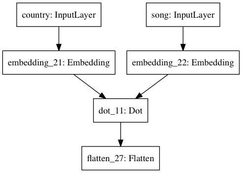
Network #1
A trivially "Siamese" network which first embeds each country and song index into $\mathbb{R}^f$ in parallel then computes a dot-product of the embeddings. This is roughly equivalent to what is being done by IMF.
country_input = Input(shape=(1,), dtype='int64', name='country')
song_input = Input(shape=(1,), dtype='int64', name='song')

country_embedding = Embedding(input_dim=n_countries, output_dim=F, embeddings_regularizer=l2(lmbda))(country_input)
song_embedding = Embedding(input_dim=n_songs, output_dim=F, embeddings_regularizer=l2(lmbda))(song_input)

predicted_preference = dot(inputs=[country_embedding, song_embedding], axes=2)
predicted_preference = Flatten()(predicted_preference)
model = Model(inputs=[country_input, song_input], outputs=predicted_preference)
model.compile(loss=implicit_cf_loss, optimizer=Adam(lr=LEARNING_RATE))

plot_model(model, to_file='figures/network_1.png')
inputs = [ratings_df['country_index'], ratings_df['song_index']]

network_1 = model.fit(
    x=inputs,
    y=ratings_df['train_rating'],
    batch_size=1024,
    epochs=5,
    validation_data=(inputs, ratings_df['validation_rating'])
)
predictions = generate_predictions(model=model, inputs=inputs)
evaluate_predictions(predictions)
For reference, let's recall the results we computed when validation our model with best_params.
grid_search_results[best_params]
Additionally, a random model should return an expected percentile ranking of ~50%, as noted in Hu, Koren and Volinksy. So, this is really bad. Let's visualize the distribution of predictions before moving on to another model.
visualize_predictions(predictions)

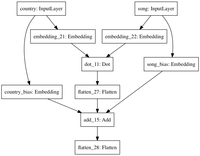
Network #2
Same as previous, but with a bias embedding for each set, in $\mathbb{R}$, added to the dot-product.
country_bias = Embedding(input_dim=n_countries, output_dim=1, name='country_bias', input_length=1)(country_input)
song_bias = Embedding(input_dim=n_songs, output_dim=1, name='song_bias', input_length=1)(song_input)

predicted_preference = add(inputs=[predicted_preference, song_bias, country_bias])
predicted_preference = Flatten()(predicted_preference)
model = Model(inputs=[country_input, song_input], outputs=predicted_preference)
model.compile(loss=implicit_cf_loss, optimizer=Adam(lr=LEARNING_RATE))

plot_model(model, to_file='figures/network_2.png')
inputs = [ratings_df['country_index'], ratings_df['song_index']]

network_2 = model.fit(
    x=inputs,
    y=ratings_df['train_rating'],
    batch_size=1024,
    epochs=5,
    validation_data=(inputs, ratings_df['validation_rating'])
)
predictions = generate_predictions(model=model, inputs=inputs)
evaluate_predictions(predictions)
This looks a lot better. Now let's visualize our ground-truth and predictions side-by-side.
_ = pd.DataFrame({
    'predictions': predictions.values.flatten(),
    'ratings': ratings_df['train_rating'].values.flatten()
}).hist(figsize=(16, 6))

This model approximates the training distribution much better than the others. Key to this task is delineating between items with 0 ratings, and those with high ratings. Remember, we first down-scaled our ratings with the following transformation to shrink the domain:
$$\tilde{r}_{u, i} = \log{\bigg(\frac{1 + r_{u, i}}{\epsilon}\bigg)}$$Furthermore, the model scores worse on the training distribution, yet similarly on the validation set. The bias term was clearly helpful.
Let's try a similar model, but concatenate the country and song embeddings, then stack fully connected layers, then compute the final linear combination as before.
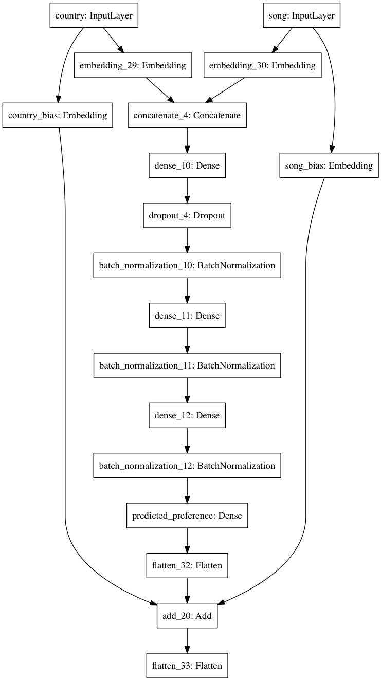
Network #3
Same as #1, but concatenate the latent vectors instead. Then, stack 3 fully-connected layers with ReLU activations, batch normalization after each, and dropout after the first. Finally, add a 1-unit dense layer on the end, and add bias embeddings to the result. (NB: I wanted to add the bias embeddings to the respective $\mathbb{R}^f$ embeddings at the outset, but couldn't figure out how to do this in Keras.)
country_input = Input(shape=(1,), dtype='int64', name='country')
song_input = Input(shape=(1,), dtype='int64', name='song')

country_embedding = Embedding(input_dim=n_countries, output_dim=F, embeddings_regularizer=l2(lmbda))(country_input)
song_embedding = Embedding(input_dim=n_songs, output_dim=F, embeddings_regularizer=l2(lmbda))(song_input)

country_bias = Embedding(input_dim=n_countries, output_dim=1, name='country_bias', input_length=1)(country_input)
song_bias = Embedding(input_dim=n_songs, output_dim=1, name='song_bias', input_length=1)(song_input)

concatenation = concatenate([country_embedding, song_embedding])

dense_layer = Dense(activation='relu', units=10)(concatenation)
dropout = Dropout(.5)(dense_layer)
batch_norm = BatchNormalization()(dropout)
dense_layer = Dense(activation='relu', units=10)(batch_norm)
batch_norm = BatchNormalization()(dense_layer)
dense_layer = Dense(activation='relu', units=10)(batch_norm)
batch_norm = BatchNormalization()(dense_layer)

predicted_preference = Dense(units=1, name='predicted_preference')(batch_norm)
predicted_preference = Flatten()(predicted_preference)

predicted_preference = add(inputs=[predicted_preference, country_bias, song_bias])
predicted_preference = Flatten()(predicted_preference)
model = Model(inputs=[country_input, song_input], outputs=predicted_preference)
model.compile(loss=implicit_cf_loss, optimizer=Adam(lr=LEARNING_RATE))

plot_model(model, to_file='figures/network_3.png')
inputs = [ratings_df['country_index'], ratings_df['song_index']]

network_3 = model.fit(
    x=inputs,
    y=ratings_df['train_rating'],
    batch_size=1024,
    epochs=5,
    validation_data=(inputs, ratings_df['validation_rating'])
)
predictions = generate_predictions(model=model, inputs=inputs)
evaluate_predictions(predictions)
These results are roughly identical to the previous. Choosing between the models, we'd certainly go with the simpler of the two.
Now, let's try some architectures that benefit from other data sources altogether: the song title, and the song artist.
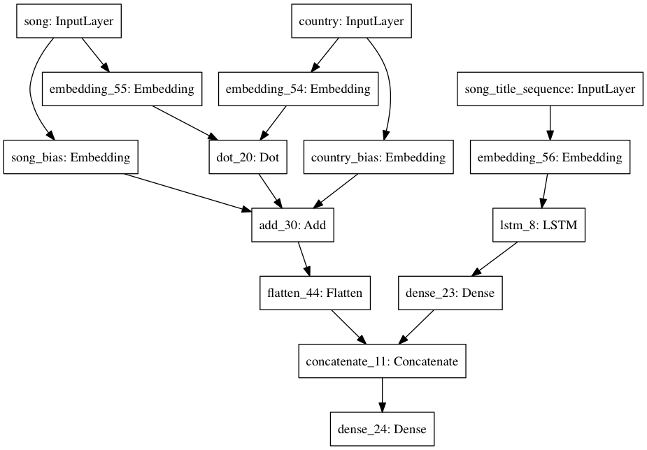
Network #4
Same as #2, except feed in the song title text as well. This text is first tokenized, then padded to a maximum sequence length, then embedded into a fixed-length vector by an LSTM, then reduced to a single value by a dense layer with a ReLU activation. Finally, this scalar is concatenated to the scalar output that #2 would produce, and the result is fed into a final dense layer with a linear activation - i.e. a linear combination of the two.
MAX_SEQUENCE_LENGTH = ratings_df['title_sequence'].map(len).max()

padded_title_sequences = pad_sequences(sequences=ratings_df['title_sequence'], maxlen=MAX_SEQUENCE_LENGTH)
country_input = Input(shape=(1,), dtype='int64', name='country')
song_input = Input(shape=(1,), dtype='int64', name='song')
title_input = Input(shape=(MAX_SEQUENCE_LENGTH,), dtype='int32', name='song_title_sequence')

country_embedding = Embedding(input_dim=n_countries, output_dim=F, embeddings_regularizer=l2(lmbda))(country_input)
song_embedding = Embedding(input_dim=n_songs, output_dim=F, embeddings_regularizer=l2(lmbda))(song_input)
title_embedding = Embedding(output_dim=F, input_dim=NUM_WORDS, input_length=MAX_SEQUENCE_LENGTH)(title_input)

country_bias = Embedding(input_dim=n_countries, output_dim=1, name='country_bias', input_length=1)(country_input)
song_bias = Embedding(input_dim=n_songs, output_dim=1, name='song_bias', input_length=1)(song_input)

predicted_preference = dot(inputs=[country_embedding, song_embedding], axes=2)
predicted_preference = add(inputs=[predicted_preference, country_bias, song_bias])
predicted_preference = Flatten()(predicted_preference)

title_lstm = LSTM(F)(title_embedding)
dense_title_lstm = Dense(units=1, activation='relu')(title_lstm)

predicted_preference_merge = concatenate(inputs=[predicted_preference, dense_title_lstm])
final_output = Dense(activation='linear', units=1)(predicted_preference_merge)
model = Model(inputs=[country_input, song_input, title_input], outputs=final_output)
model.compile(loss=implicit_cf_loss, optimizer=Adam(lr=LEARNING_RATE))

plot_model(model, to_file='figures/network_4.png')
inputs = [ratings_df['country_index'], ratings_df['song_index'], padded_title_sequences]

network_4 = model.fit(
    x=inputs,
    y=ratings_df['train_rating'],
    batch_size=1024,
    epochs=5,
    validation_data=(inputs, ratings_df['validation_rating'])
)
predictions = generate_predictions(model=model, inputs=inputs)
evaluate_predictions(predictions)
We seem to get a pinch of lift from the song title, though we're still underfitting our training set. Perhaps we could make our model bigger, or run it for more epochs.
Let's plot our ground-truth vs. prediction distributions side-by-side just to make sure we're still on the right track.
_ = pd.DataFrame({
    'predictions': predictions.values.flatten(),
    'ratings': ratings_df['train_rating'].values.flatten()
}).hist(figsize=(16, 6))

Finally, let's add the artist.
Network #5
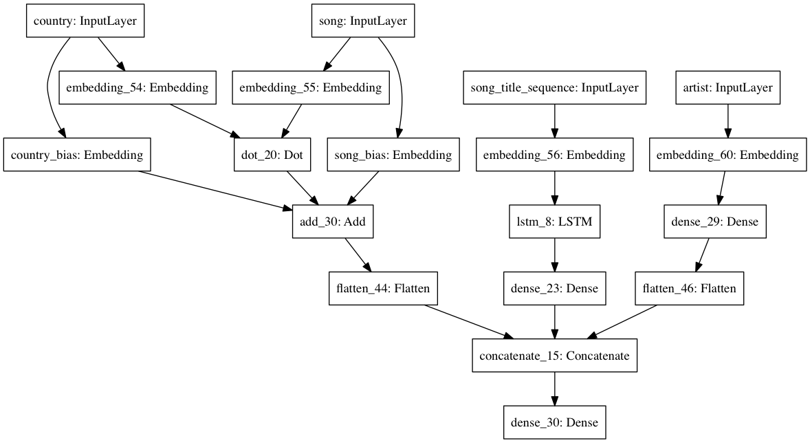
Same as #4, except feed in the song artist index as well. This index is first embedded into a vector, then reduced to a scalar by a dense layer with a ReLU activation. Finally, this scalar is concatenated with the two scalars produced in the second-to-last layer of #4, then fed into a final dense layer with a linear activation. Like the previous, this is a linear combination of the three inputs.
artist_input = Input(shape=(1,), dtype='int64', name='artist')
artist_embedding = Embedding(input_dim=n_artists, output_dim=F, embeddings_regularizer=l2(lmbda))(artist_input)
dense_artist_embedding = Dense(units=1, activation='relu')(artist_embedding)
dense_artist_embedding = Flatten()(dense_artist_embedding)

predicted_preference_merge = concatenate(inputs=[predicted_preference, dense_title_lstm, dense_artist_embedding])
final_output = Dense(activation='linear', units=1)(predicted_preference_merge)
model = Model(inputs=[country_input, song_input, title_input, artist_input], outputs=final_output)
model.compile(loss=implicit_cf_loss, optimizer=Adam(lr=LEARNING_RATE))

plot_model(model, to_file='figures/network_5.png')
inputs = [
    ratings_df['country_index'],
    ratings_df['song_index'],
    padded_title_sequences,
    ratings_df['song_artist_index']
]

model.fit(
    x=inputs,
    y=ratings_df['train_rating'],
    batch_size=1024,
    epochs=5,
    validation_data=(inputs, ratings_df['validation_rating'])
)
predictions = generate_predictions(model=model, inputs=inputs)
evaluate_predictions(predictions)
This seems a bit worse than the last, though similar all the same. I'm a bit surprised we didn't get more lift from artists. Nevertheless, we're still underfitting. Bigger model, more epochs, etc.
country_input = Input(shape=(1,), dtype='int64', name='country')
song_input = Input(shape=(1,), dtype='int64', name='song')

country_embedding = Embedding(input_dim=n_countries, output_dim=F, embeddings_regularizer=l2(lmbda))(country_input)
song_embedding = Embedding(input_dim=n_songs, output_dim=F, embeddings_regularizer=l2(lmbda))(song_input)

country_bias = Embedding(input_dim=n_countries, output_dim=1, name='country_bias', input_length=1)(country_input)
song_bias = Embedding(input_dim=n_songs, output_dim=1, name='song_bias', input_length=1)(song_input)

predicted_preference = dot(inputs=[country_embedding, song_embedding], axes=2)
predicted_preference = Flatten()(predicted_preference)

predicted_preference = add(inputs=[predicted_preference, song_bias, country_bias])
predicted_preference = Flatten()(predicted_preference)
model = Model(inputs=[country_input, song_input], outputs=predicted_preference)
model.compile(loss=implicit_cf_loss, optimizer=Adam(lr=LEARNING_RATE))
inputs = [ratings_df['country_index'], ratings_df['song_index']]

network_2 = model.fit(
    x=inputs,
    y=ratings_df['train_rating'],
    batch_size=1024,
    epochs=5,
    validation_data=(inputs, ratings_df['validation_rating'])
)
predictions = generate_predictions(model=model, inputs=inputs)
evaluate_predictions(predictions)
predictions_unstack = predictions.unstack()

predictions_unstack = pd.DataFrame({
    'song_title': song_metadata_df.ix[predictions_unstack.index.get_level_values('song_id')]['song_title'],
    'song_artist': song_metadata_df.ix[predictions_unstack.index.get_level_values('song_id')]['song_artist'],
    'country': unstack.index.get_level_values('country_id').map(country_id_to_name.get),
    'rating': predictions_unstack.values
})
Colombia
predictions_unstack[predictions_unstack['country'] == 'Colombia'].sort_values(by='rating', ascending=False).head(10)
United States
predictions_unstack[predictions_unstack['country'] == 'United States'].sort_values(by='rating', ascending=False).head(10)
Turkey
predictions_unstack[predictions_unstack['country'] == 'Turkey'].sort_values(by='rating', ascending=False).head(10)
Taiwan
predictions_unstack[predictions_unstack['country'] == 'Taiwan'].sort_values(by='rating', ascending=False).head(10)
As is abundantly clear, the model is simply converging to a popularity baseline. I tried extracting the vectors outright, normalizing as before then computing dot products, but the results made little sense.
Future work
At this stage, Implicit Matrix Factorization is the clear winner. The algorithm is popular for several good reasons - it's simple, relatively scalable, intuitive (especially given the significance of the interplay between $C$ and $P$, which I did not expressedly discuss) and effective. Herein, I did not produce a neural network approximating this algorithm with superior results.
My intuition tells me I'm missing something simple; why shouldn't a non-linear function approximator be able to approximate $f(u, i)$ better than a linear matrix decomposition? At this stage, I'm not sure. My best guess is that we should seek to optimize a different loss function. Here, we've mirrored that of IMF; why not optimize a ranking loss function instead, since that's what's ultimately important? The IMF objective makes the actual optimization process easy for ratings matrices with billions of items; in our case, with far fewer items, we're simply using stochastic gradient descent. To this effect, I did experiment with some composite loss functions; on one side, implicit_mf_loss, and on the other, a cutoff_loss, which seeks to enforce that songs which received a rating $\tilde{r}_{u, i}$ above a certain cutoff should be indeed predicted at above that cutoff. It's a crude, binary absolute error. This was unsuccessful.
Finally, if there is in fact some value in using neural networks for this type of problem, I'm extremely intrigued by the ease and intuitiveness with which we can incorporate multiple inputs into our function. Encoding our song title with an LSTM, and training that LSTM end-to-end with our main minimization objective, is one example of this. Furthermore, Keras makes the construction of these networks straightforward.
Thanks for reading this work. Your feedback is welcome, and I do hope this serves as a point of inspiration, trial and error should this question interest you.