I recently finished a course on discrete optimization and am currently working through Richard McElreath's excellent textbook Statistical Rethinking. Combining the two, and duly jazzed by this video on the Traveling Salesman Problem, I'd thought I'd build a toy Bayesian model and try to optimize it via simulated annealing.
This work was brief, amusing and experimental. The result is a simple Shiny app that contrasts MCMC search via simulated annealing versus the (more standard) Metropolis algorithm. While far from groundbreaking, I did pick up the following few bits of intuition along the way.
A new favorite analogy for Bayesian inference
I like teaching things to anyone who will listen. Fancy models are useless if your boss doesn't understand. Simple analogies are immensely effective for communicating almost anything at all.
The goal of Bayesian inference is, given some data, to figure out which parameters were employed in generating that data. The data itself come from generative processes - a Binomial process, a Poisson process, a Normal process (as is used in this post), for example - which each require parameters to get off the ground (in the same way that an oven needs a temperature and a time limit before it can start making bread) - \(n\) and \(p\); \(\lambda\); \(\mu\) and \(\sigma\), respectively. In statistical inference, we work backwards: we're given the data, we hypothesize from which type of process(es) it was generated, and we then do our best to guess what these initial parameters were. Of course, we'll never actually know: if we did, we wouldn't need to do any modeling at all.
Bayes' theorem is as follows:
Initially, all we have is \(X\): the data that we've observed. During inference, we pick a parameter value \(p\) - let's start with \(p = 123\) - and compute both \(P(X | p)\) and \(P(p)\). We then multiply these two together, leaving us with an expression of how likely \(p\) is to be the real parameter that was initially plugged into our generative process (that then generated the data we have on hand). This expression is called the posterior probability (of \(p\), given \(X\)).
The centerpiece of this process is the computation of the quantities \(P(X | p)\) and \(P(p)\). To understand, let us use the example of vetting, i.e. vetting an individual applying for citizenship in your country - a typically multi-step process. In this particular vetting process, there are two steps.
-
The first step, and perhaps the "broader stroke" of the two, is the prior probability of this parameter. In setting up our problem we choose a prior distribution - i.e. our a priori belief of the possible range of values this true parameter \(p\) can take - and the prior probability \(P(p)\) echoes how likely we thought \(p = 123\) to be the real thing before we saw any data at all.
-
The second step is the likelihood of our data given this parameter. It says: "assuming \(p = 123\) is the real thing, how likely was it to have observed the data that we did?" For further clarity, let's assume in an altogether different problem that our data consists of 20 coin-flips - 17 heads, and 3 tails - and the parameter we're currently vetting is \(p_{heads} = .064\) (where \(p_{heads}\) is the probability of flipping "heads"). So, "assuming \(p = .064\) is the real thing, how likely was it to have observed the data that we did?" The answer: "Err, not likely whatsoever."
Finally, we multiply these values together to obtain the posterior probability, or the "yes admit this person into the country" score. If it's high, they check out.
Computing the posterior on the log scale is important
The prior probability \(P(p)\) for a given parameter is a single floating point number. The likelihood of a single data point \(x\) given that parameter \(p\), expressed \(P(x | p)\), is a single floating point number. To compute the likelihood of all of our data \(X\) given that parameter \(p\), expressed \(P(X | p)\), we must multiply the individual likelihoods together - one for each data point. For example, if we have 100 data points, \(P(X | p)\) is the product of 100 floating point numbers. We can write this compactly as:
Likelihood values are often pretty small, and multiplying small numbers together makes them even smaller. As such, computing the posterior on the log scale allows us to add instead of multiply, which solves some numerical precision troubles that computers often have. With 100 data points, computing the log posterior would be a sum of 101 numbers. On the natural scale, the posterior would be the product of 101 numbers.
Optimization is a thing
I used to get easily frustrated with oft-used big words that I personally felt conferred no meaning whatsoever. "Optimization," for example: "We here at XYZ Consulting undertake optimal processes for maximal profit." Optimal, eh? What does that actually mean?
In recent months, I've realized optimization is just a collection of strategies for finding intelligent and warm-hearted prospective citizens: specifically, given one prospective citizen (parameter) that is sufficiently terrific (has a high posterior probability given the data we've observed), how do we then find a bunch more? In the discrete world, simulated annealing, mixed-integer programming, branch and bound, etc. would be a few of these strategies. In the continuous world, gradient descent, L-BFGS, the Powell algorithm and brute-force grid search are a few such examples.
In most mathematical cases, the measure of "sufficiently terrific" refers to a good score on a relevant loss function. In the case of XYZ Consulting, this metric is certainly more vague. (And while there may be some complex numerical optimization routine guiding their decisions, well, I'd guess the PR-score is the metric they're more likely after.)
Findings
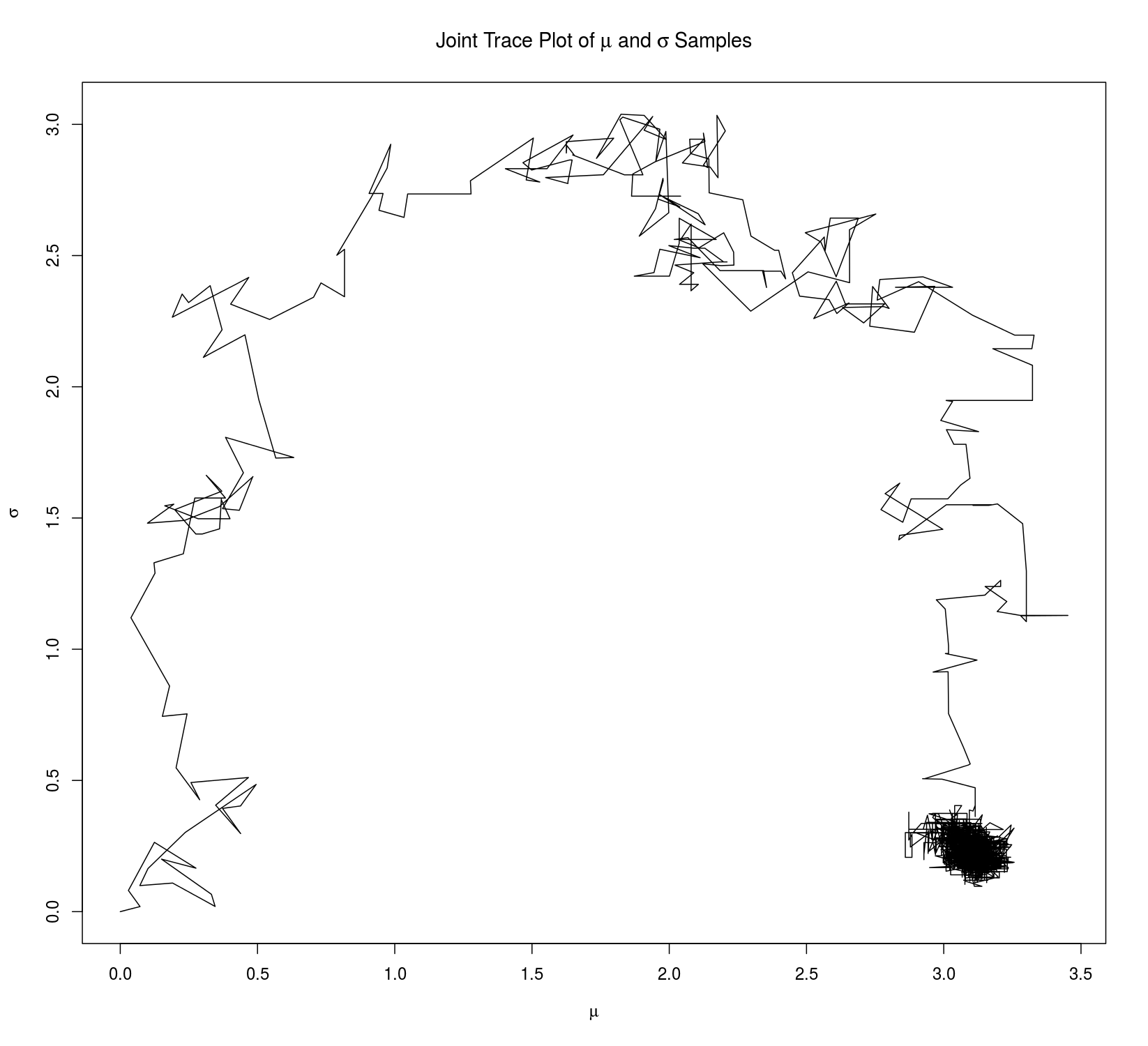
The most salient difference between the simulated annealing and Metropolis samplers is the "cooling schedule" of the former. In effect, simulated annealing becomes fundamentally more "narrow-minded" as time goes on: it finds a certain type of prospective citizen it likes, and it thereafter goes searching only for others that are very close in nature. Concretely, with a very quick cooling schedule, this can result in a skinny and tall posterior; when using simulating annealing for MCMC, we must take care to use a schedule that allows for sufficient exploration of the parameter space. With the Metropolis sampler, we don't have this problem.
Finally, I've found that I quite enjoy using R. Plotting is miles easier than in Python and the pipe operators aren't so bad.
Thanks a lot for reading.
Code:
The code for this project can be found here.