RescueTime Inference via the "Poor Man's Dirichlet"

RescueTime is "a personal analytics service that shows you how you spend your time [on the computer], and provides tools to help you be more productive." Personally, I've been a RescueTime user since late-January 2016, and while it does ping me guilty for harking back to a dangling Facebook tab in Chrome, I haven't yet dug much into the data it's thus-far stored.

In short, I built a Shiny app that estimates my/your typical week with RescueTime. In long, the analysis is as follows.

The basic model of RescueTime is thus: track all activity, then categorize this activity by both "category" — "Software Development," "Reference and Learning," "Social Learning," etc. — and "productivity level" — "Very Productive Time," "Productive Time," "Neutral Time," "Distracting Time" and "Very Distracting Time." For example, 10 minutes spent on Twitter would be logged as (600 seconds, "Social Networking", "Very Distracting Time"), while 20 minutes on an arxiv paper logged as (1200 seconds, "Reference & Learning," "Very Productive Time"). Finally, RescueTime maintains (among other minutia) an aggregate "productivity score" by day, week and year.

The purpose of this post is to take my weekly summary for 2016 and examine how I'm doing thus far. More specifically, with a dataset containing the total seconds-per-week spent [viewing resources categorized] at each of the 5 distinct productivity levels, I'd like to infer the productivity breakdown of a typical week. Rows of this dataset — after dividing all values in each by its sum — will contain 5 numbers, with each expressing the percentage of that week spent at the respective productivity level. Examples might include: \((.2, .3, .1, .2, .2)\), \((.1, .3, .2, .15, .25)\) or \((.05, .25, .3, .25, .15)\). Of course, the values in each row must sum to 1.

In effect, we can view each row as an empirical probability distribution over the 5 levels at hand. As such, our goal is to infer the process that generated these samples in the first place. In the canonical case, this generative process would be a Dirichlet distribution — a thing that takes a vector \(\alpha\) and returns vectors of the length of \(\alpha\) containing values that sum to 1. With a Dirichlet model conditional on the RescueTime data observed, the world becomes ours: we can generate new samples (a "week" of RescueTime log!) ad infinitum, ask questions of these samples (e.g. "what percentage of the time can we expect to log more 'Very Productive Time' than 'Productive Time?'"), and get some proxy lens into the brain cells and body fibers that spend our typical week in front of the computer in the manner that they do.

To begin this analysis, I first download the data at the following link. If you're not logged in, you'll be first prompted to do so. To do the same, you must be a paying RescueTime user. If you're not, you're welcome to use my personal data in order to follow along.

The data at hand have 48 rows. First, let's see what they look like.

> head(report)
 week very_distracting distracting neutral productive very_productive
1 2016-01-31T00:00:00 0.05802495 0.15878213 0.1179268 0.05471899 0.6105471
2 2016-02-07T00:00:00 0.16082036 0.11625240 0.1251466 0.06762928 0.5301514
3 2016-02-14T00:00:00 0.07335485 0.18299335 0.1269896 0.08361825 0.5330439
4 2016-02-21T00:00:00 0.07911463 0.04051227 0.1445033 0.05395296 0.6819169
5 2016-02-28T00:00:00 0.07513117 0.12542957 0.1560940 0.04884047 0.5945047
6 2016-03-06T00:00:00 0.04554125 0.12288119 0.1410541 0.08958757 0.6009359

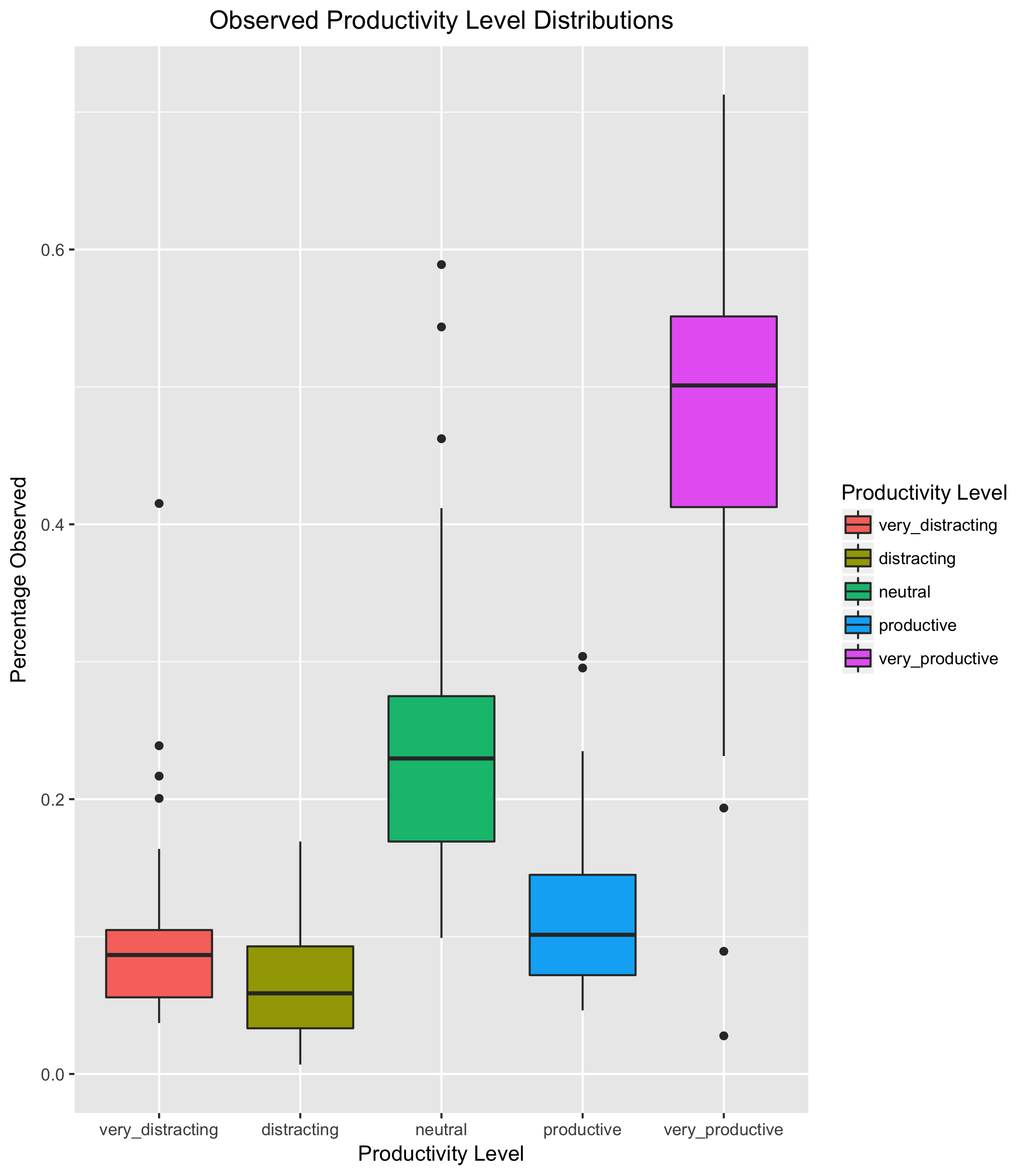
Next, let's see how each level is distributed:

Finally, let's choose a modeling approach. Once more, I venture that each week should be viewed as a draw from a Dirichlet distribution; at the very least, no matter how modeled, each week (draw) is inarguably a vector of values that sum to 1. To this effect, I see a few possible approaches.

Dirichlet Process

A Dirichlet Process (DP) is a model of a distribution over distributions. In our example, this would imply that each week's vector is drawn from one of several possible Dirichlet distributions, each one governing a fundamentally different type of week altogether. For example, let's posit that we have several different kinds of work weeks: a "lazy" week, a "fire-power-super-charged week," a "start-slow-finish-strong week," a "cram-all-the-things-on Friday week." Each week, we arrive to work on Monday morning and our aforementioned brain cells and body fibers "decide" what type of week we're going to have. Finally, we play out the week and observe the resulting vector. Of course, while two weeks might have the same type, the resulting vectors will likely be (at least) slightly different.

In this instance, given a Dirichlet Process \(DP(G_0, \alpha)\) — where \(G_0\) is the base distribution (from which the cells and fibers decide what type of week we'll have) and \(\alpha\) is some prior — we first draw a week-type distribution from the base, then draw our week-level probability vector from the result. As a bonus, a DP is able to infer an infinite number of week-type distributions from our data (as compared to K-Means, for example, in which we would have to specify this value a priori) which fits nicely with the problem at hand: à la base, how many distinct week-types do we truly have? How would we ever know?

Dirichlet Processes are best understood through one of several simple generative statistical processes, namely the Chinese Restaurant Process, Polya Urn Model or Stick-Breaking Process. Edwin Chen has an excellent post dissecting each and its relation to the DP itself.

Dirichlet Inference via Conjugacy

Given that a Dirichlet distribution is an exponential model, "all members of the exponential family have conjugate priors"¹ and our data can be intuitively viewed as Dirichlet draws, it would be fortuitous if there existed some nice algebraic conjugacy to make inference a breeze. We know how to use Beta-Binomial and Dirichlet-Multinomial, but unfortunately there doesn't seem to be much in the way of X-Dirichlet². As such, this approach unfortunately dead-ends here.

The "Poor-Man's Dirichlet" via Linear Models

A final approach has us modeling the mean of each productivity-level proportion \(\mu_i\) as:

For each \(\phi_j\), we place a normal prior \(\phi_j \sim \text{Normal}(\mu_j, \sigma_j)\), and finally give the likelihood of each productivity-level proportion \(p_i\) as \(p_i \sim \text{Normal}(\mu_i, \sigma)\) as in the canonical Bayesian linear regression. There's two key points to make on this approach.

1. As each \(\mu_i\) is given by the softmax function the values \(\phi_j\) are not uniquely identifiable, i.e. softmax(vector) = softmax(100 + vector). In other words, because the magnitude of the values \(\phi_j\) (how big they are) is unimportant, we cannot (nor do we need to) solve for these values exactly. I like to think of this as inference on two multi-collinear variables in a linear regression: with \(corr(x_1, x_2) \approx 1\), we can re-express our regression \(\mu = \alpha + \beta_1 x_1 + \beta_2 x_2\) as \(\mu = \alpha + (\beta_1 + \beta_2)x_1\); in effect, we now have only 1 coefficient to solve for, and while the sum \(\beta_1 + \beta_2\) is what we're trying to infer, the individual values \(\beta_1\) and \(\beta_2\) are of no importance. (For example, if \(\beta_1 + \beta_2 = 10\), we could choose \(\beta_1 = 3\) and \(\beta_2 = 7\), or \(\beta_1 = 9\) and \(\beta_2 = 1\), or \(\beta_1 = .01\) and \(\beta_2 = 9.99\) to no material difference.) In this case, while interpretation of the individual coefficients \(\beta_1\) and \(\beta_2\) would be erroneous, we can still make perfectly sound predictions on \(\mu\) with the posterior for \(\beta_1 + \beta_2\). To close, this is but a tangential way of saying that while the posteriors of each individual \(\phi_j\) will be of little informative value, the softmax itself will still work out just fine.

2. I've chosen the likelihood as the normal distribution with respective means \(\mu_i\) and a shared standard deviation \(\sigma\). First, I note that I hope this is the correct approach, i.e. "do it like you would with a typical linear model." Second, I chose a shared standard deviation (and, frankly, prayed it would be small) as my aim was to omit it from analysis/posterior prediction entirely: while simulating \(\mu_i\) seems perfectly sound, making a draw from the likelihood function, i.e. the normal distribution with mean \(\mu_i\) and standard deviation \(\sigma\), would cause our simulated productivity-level proportions to no longer add up to 1! This seems like the worst of all evils. While the spread of the respective distributions does seem to vary — thus suggesting we would be wise to infer a separate \(\sigma_i\) for each — I chose to brush this fact aside because: one, the \(p_i\)'s are not independent, i.e. as one goes up another must necessarily go down, which I hoped might be in some way "captured" by the single parameter, and two, I didn't intend to use the \(\sigma\) posterior in the analysis for the reason mentioned above, checking only to see that it converged.

In the end, I chose Option 3 for a few simple reasons. First, I have no reason to believe that the data were generated by a variety of distinct "week-type" distributions; a week is a rather large unit of time. In addition, the spread of the empirical distributions don't appear, by no particularly rigorous measure, that erratic. Conversely, if this were instead day-level data, this argument would be much more plausible and the data would likely corroborate this point. Second, Gelman suggests this approach in response to a similar question, adding "I’ve personally never had much success with Dirichlets."²

To build this model, I elect to use Stan in R, defining it as follows:

data {
 int<lower=1> N;
 real very_distracting[N];
 real distracting[N];
 real neutral[N];
 real productive[N];
}

parameters {
 real phi_a;
 real phi_b;
 real phi_c;
 real phi_d;
 real phi_e;
 real<lower=0, upper=1> sigma;
}

transformed parameters {
 real mu_a;
 real mu_b;
 real mu_c;
 real mu_d;
 mu_a = exp(phi_a) / ( exp(phi_a) + exp(phi_b) + exp(phi_c) + exp(phi_d) + exp(phi_e) );
 mu_b = exp(phi_b) / ( exp(phi_a) + exp(phi_b) + exp(phi_c) + exp(phi_d) + exp(phi_e) );
 mu_c = exp(phi_c) / ( exp(phi_a) + exp(phi_b) + exp(phi_c) + exp(phi_d) + exp(phi_e) );
 mu_d = exp(phi_d) / ( exp(phi_a) + exp(phi_b) + exp(phi_c) + exp(phi_d) + exp(phi_e) );
}

model {
 sigma ~ uniform( 0 , 1 );
 phi_a ~ normal( 0 , 1 );
 phi_e ~ normal( 0 , 1 );
 phi_d ~ normal( 0 , 1 );
 phi_c ~ normal( 0 , 1 );
 phi_b ~ normal( 0 , 1 );
 very_distracting ~ normal(mu_a, sigma);
 distracting ~ normal(mu_b, sigma);
 neutral ~ normal(mu_c, sigma);
 productive ~ normal(mu_d, sigma);
}

Here (with a, b, c, d, e corresponding respectively to "Very Distracting Time," "Distracting Time," "Neutral," "Productive Time," "Very Productive Time") I model the likelihoods of all but e, as this can be computed deterministically from the posterior samples of a, b, c and d as \(e = 1 - a - b - c - d\). For priors, I place \(\text{Normal}(0, 1)\) priors on \(\phi_j\), the magnitude of which should be practically irrelevant as stated previously. Finally, I give \(\sigma\) a \(\text{Uniform}(0, 1)\) prior, which seemed like a logical magnitude for mapping a vector of values that sum to 1 to another vector of values that sum (to something close to) to 1.

Instinctually, this modeling framework seems like it might have a few leaks in the theoretical ceiling — especially with respect to my choices surrounding the shared \(\sigma\) parameter. Should you have some feedback on this approach, please do drop a line in the comments below.

To fit the model, I use the standard Stan NUTS engine to build 4 MCMC chains, following Richard McElreath's "four short chains to check, one long chain for inference!"³. The results — fortunately, quite smooth — are as follows:

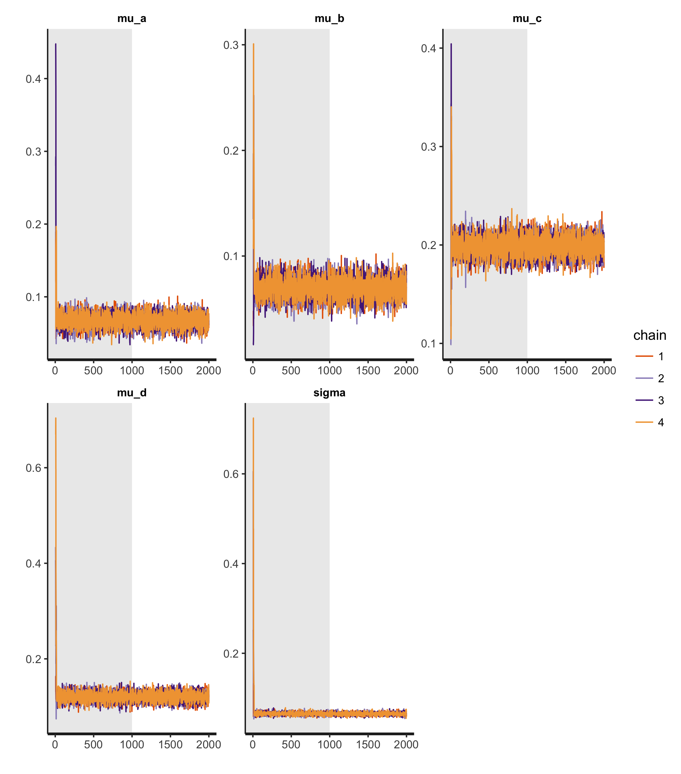
The gray area of the plot pertains to the warmup period, while the white gives the valid samples. All four chains appear highly-stationary, well-mixing and roughly identical. Finally, let's examine the convergence diagnostics themselves:

Inference for Stan model: model.
4 chains, each with iter=2000; warmup=1000; thin=1;
post-warmup draws per chain=1000, total post-warmup draws=4000.

      mean se_mean   sd 1.5% 98.5% n_eff Rhat
mu_a  0.07       0 0.01 0.05  0.09  4000    1
mu_b  0.07       0 0.01 0.05  0.09  4000    1
mu_c  0.20       0 0.01 0.18  0.22  4000    1
mu_d  0.12       0 0.01 0.10  0.14  4000    1
sigma 0.07       0 0.00 0.06  0.07  1792    1

Both Rhat — a value which we hope to equal 1, would be "suspicious at 1.01 and catastrophic at 1.10"³ — and n_eff — which expresses the "effective" number of samples, i.e. the samples not discarded due to high autocorrelation in the NUTS process — are right where we want them to be. Furthermore, \(\sigma\) ends up being rather small, and with a rather-tight 97% prediction interval to boot.

Next, let's draw 2000 samples from the joint posterior and plot the respective distributions of \(\mu_i\) against one another:

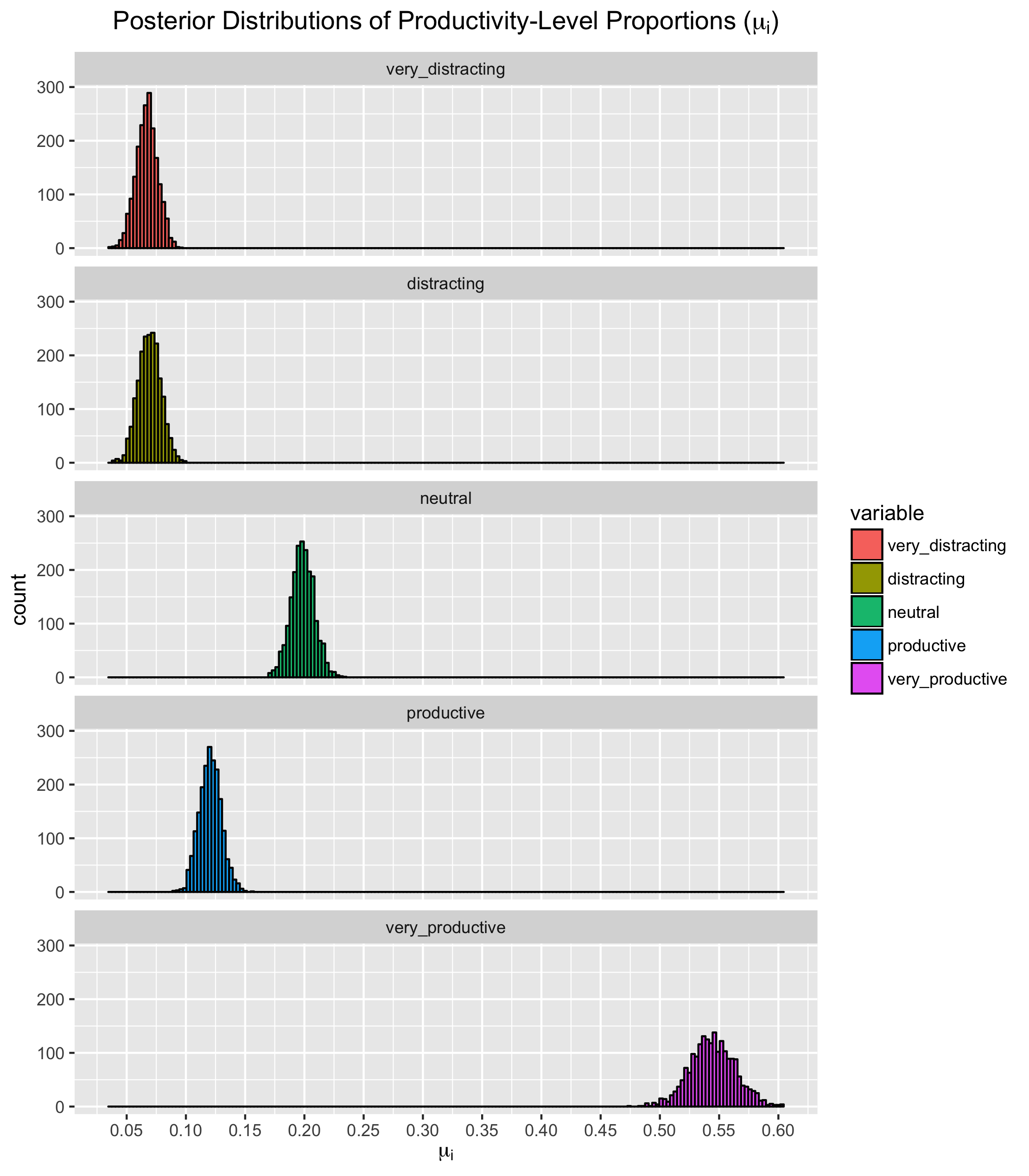
Remember, the above posterior distributions are for the expected values (mean) of each productivity-level proportion. In our model, we then insert this mean into a normal distribution (the likelihood function) with standard deviation \(\sigma\) and draw our final value.

Finally, let's compute the mean of each posterior for a final result:

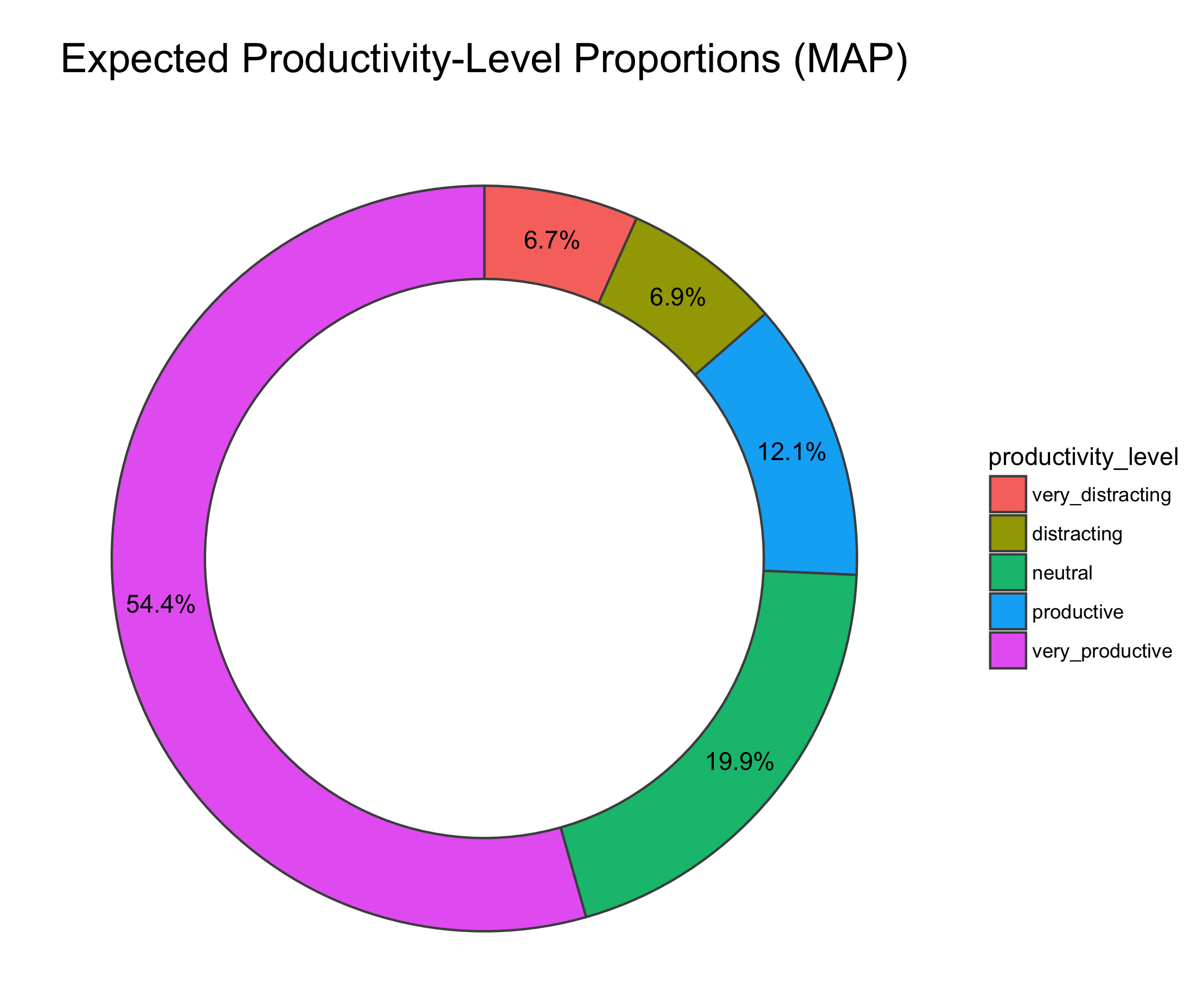
In summary, I've got work to do. Time to cast off those "Neutral" clothes and toss it to the purple.

Additional Resources:

1. More MCMC – Analyzing a small dataset with 1-5 ratings

Code:

The code for this project can be found here.