In my experience, the gap between a conceptual understanding of how a machine learning model "learns" and a concrete, "I can do this with a pencil and paper" understanding is large. This gap is further exacerbated by the nature of popular machine learning libraries which allow you to use powerful models without knowing how they really work. This isn't such a bad thing. But knowledge is power. In this post, I aim to close the gap above for a vanilla neural network that learns by gradient descent: we will use gradient descent to learn a weight and a bias for a single neuron. From there, when learning an entire network of millions of neurons, we just do the same thing a bunch more times. The rest is details. The following assumes a cursory knowledge of linear combinations, activation functions, cost functions, and how they all fit together in forward propagation. It is math-heavy with some Python interspersed.
Problem setup
Our neuron looks like this:
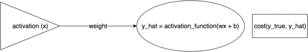
Our parameters look like this:
ACTIVATION = 3
INITIAL_WEIGHT = .5
INITIAL_BIAS = 2
ACTUAL_OUTPUT_NEURON_ACTIVATION = 0
N_EPOCHS = 5000
LEARNING_RATE = .05
Let's work backwards
We have an initial weight and bias of:
weight = 3
bias = 2
After each iteration of gradient descent, we update these parameters via:
weight += -LEARNING_RATE * weight_gradient
bias += -LEARNING_RATE * bias_gradient
This is where the "learning" is concretized: changing a weight and a bias to a different weight and bias that makes our network better at prediction. So: how do we obtain the weight_gradient and bias_gradient? More importantly, why do we want these things in the first place?
Why we want the gradient
I'll be keeping this simple because it is simple. Our initial weight (\(w_0 = 3\)) and bias (\(b_0 = 2\)) were chosen randomly. As such, our network will likely make terrible predictions. By definition, our cost will be high. We want to make our cost low. Let's pick a new weight and bias that change this cost by \(\Delta C\), where \(\Delta C\) is some strictly negative number. For our weight: Define \(\Delta C\) as "how much our cost changes with respect to a 1 unit change in our weight" times "how much we changed our weight". In math, that looks like:
Our goal is to make \(\Delta C\) strictly negative, such that every time we update our weight, we do so in a way that lowers our cost. Duh. Let's choose \(\Delta w = -\eta\ \nabla C\). Our previous expression becomes:
\(\|\nabla C\|\) is strictly positive, and a positive number multiplied by a negative number (\(-\eta\)) is strictly negative. So, by choosing \(\Delta w = -\eta\ \nabla C\), our \(\Delta C\) is always negative; in other words, at each iteration of gradient descent - in which we perform weight += delta_weight, a.k.a. weight += -LEARNING_RATE * weight_gradient - our cost always goes down. Nice.
For our bias, it's the very same thing.
Deriving \(\frac{\partial C}{\partial w}\) and \(\frac{\partial C}{\partial b}\)
Deriving both \(\frac{\partial C}{\partial w}\) and \(\frac{\partial C}{\partial b}\) is pure 12th grade calculus. Plain and simple. If you forget your 12th grade calculus, spend ~2 minutes refreshing your memory with an article online. It's not difficult. Before we begin, we must first define a cost function and an activation function. Let's choose quadratic loss and a sigmoid respectively.
where \(\hat{y}\) is the neuron's final output, \(z\) is the linear combination (\(wx+b\)) input, and \(\hat{y} = \sigma(z)\).
Using the chain rule, our desired expression \(\frac{\partial C}{\partial w}\) becomes:
For our bias, the expression \(\frac{\partial C}{\partial b}\) is almost identical:
Now we need expressions for \(C'\) and \(\sigma'\). Let's derive them.
As such, our final expressions for \(\frac{\partial C}{\partial w}\) and \(\frac{\partial C}{\partial b}\) are:
From there, we just plug in our values from the start (\(x\) is our ACTIVATION) to solve for weight_gradient and bias gradient. The result of each is a real-valued number. It is no longer a function, nor expression, nor nebulous mathematical concept.
Finally, as initially prescribed, we update our weight and bias via:
weight += -LEARNING_RATE * weight_gradient
bias += -LEARNING_RATE * bias_gradient
Because \(\Delta C = -\eta\|\nabla C\|\), the resulting weight and bias will give a lower cost than before. Nice!
Code:
Here's a notebook showing this process in action. Happy gradient descent.