So You Want to Implement a Custom Loss Function?

It's often not so hard.

My venerable boss recently took a trip to Amsterdam. As we live in New York City, he needed to board a plane. Days before, we discussed the asymmetric risk of airport punctuality: "if I get to the gate early, it's really not so bad; if I arrive too late and miss my flight, it really, really sucks." When deciding just when to leave the house - well - machine learning can help.

Let's assume we have a 4-feature dataset, X. In order, each columns denotes: a binary "holiday/no-holiday", a binary "weekend/no-weekend", a normalized continuous value dictating "how does the traffic on my route compare to the average day of traffic on this route", and the number of seats on the plane. Each observation is paired with a response, y, where \(y = 0\) indicates the flight will leave on time, and \(y = 1\) indicates the flight will leave later (meaning we can arrive later ourselves).

As mentioned, missing a plane is bad. You incur stress. You have to book another ticket, which is often inconveniently expensive. You have to eat your next 2 meals in the airport, which is a whole other bag of misery. If we want to train a learning algorithm to predict flight delay - and therefore inform us as to when to leave the house - we'll have to teach it just how bad the Terminal 3 beef and broccoli really is.

To train a supervised learning algorithm, we need a few things.

1. Some training data.
2. A model. Let's choose logistic regression. It's simple, deterministic, and interpretable.
3. A loss function - also known as a cost function - which quantitatively answers the following: "The real label was 1, but I predicted 0: is that bad?" Answer: "Yeah. That's bad. That's .. 500 bad." Many supervised algorithms come with standard loss functions in tow. SVM likes the hinge loss. Logistic regression likes log loss, or 0-1 loss. Because our loss is asymmetric - an incorrect answer is more bad than a correct answer is good - we're going to create our own.
4. A way to optimize our loss function. This is just a fancy way of saying: "Look. We have these 4 factors that advise us as to whether or not that airplane is going to take off on time. And we saw what happened in the past. So what we really want to know is: if it's a holiday, is our plane more or less likely to stay on schedule? How about a weekend? Does the traffic have any impact? What about the size of the plane? Finally, once I know this - once I know how each of my variables relates to the thing I'm trying to predict - I want to keep the real world in mind: 'the plane left on time, but I showed up late: is that bad?'"

To do this, we often employ an algorithm called gradient descent (and its variants), which is quick, effective, and easy to understand. Gradient descent requires we take the gradient - or derivative - of our loss function. With most typical loss functions (hinge loss, least squares loss, etc.), we can easily differentiate with a pencil and paper. With more complex loss functions, we often can't. Why not get a computer to do it for us, so we can move onto the fun part of actually fitting our model?

Introducing autograd.

Autograd is a pure Python library that "efficiently computes derivatives of numpy code" via automatic differentiation. Automatic differentiation exploits the calculus chain rule to differentiate our functions. In fact, for the purposes of this post, the implementation details aren't that important. What is important, though, is how we can use it: with autograd, obtaining the gradient of your custom loss function is as easy as custom_gradient = grad(custom_loss_function). It's really that simple.

Let's return to our airplane. We have some data - with each column encoding the 4 features described above - and we have our corresponding target. (In addition, we initialize our weights to 0, and define an epsilon with which to clip our predictions in (0, 1)).

X = np.array([
    [ 0.3213, 0.4856, 0.2995, 2.5044],
    [ 0.3005, 0.4757, 0.2974, 2.4691],
    [ 0.5638, 0.8005, 0.3381, 2.3102],
    [ 0.5281, 0.6542, 0.3129, 2.1298],
    [ 0.3221, 0.5126, 0.3085, 2.6147],
    [ 0.3055, 0.4885, 0.289 , 2.4957],
    [ 0.3276, 0.5185, 0.3218, 2.6013],
    [ 0.5313, 0.7028, 0.3266, 2.1543],
    [ 0.4728, 0.6399, 0.3062, 2.0597],
    [ 0.3221, 0.5126, 0.3085, 2.6147]
])
y = np.array([1., 1., -1., -1., 1., 1., 1., -1., -1., -1.])

weights = np.zeros(X.shape[1])
eps = 1e-15

We have our model:

def wTx(w, x):
   return np.dot(x, w)

def sigmoid(z):
   return 1./(1+np.exp(-z))

def logistic_predictions(w, x):
   predictions = sigmoid(wTx(w, x))
   return predictions.clip(eps, 1-eps)

And we define our loss function. Here, I've decided on a variant of log loss, with the latter logarithmic term exponentiated and the sign reversed. In English, it says: "If the flight actually leaves on time, and we predict that it leaves on time (and leave our house early enough), then all is right with the world. However, if we instead predict that it will be delayed (and leave our house 30 minutes later), then we'll be stressed, -$1000, and dining on rubber for the following few hours.

def custom_loss(y, y_predicted):
    return -(y*np.log(y_predicted) - (1-y)*np.log(1-y_predicted)**2).mean()

def custom_loss_given_weights(w):
    y_predicted = logistic_predictions(w, X)
    return custom_loss(y, y_predicted)

Let's see what this function looks like, for each of \(y = 1\) and \(y = 0\), and varying values of y_hat.

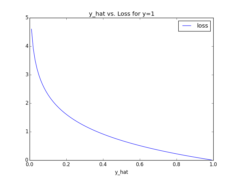
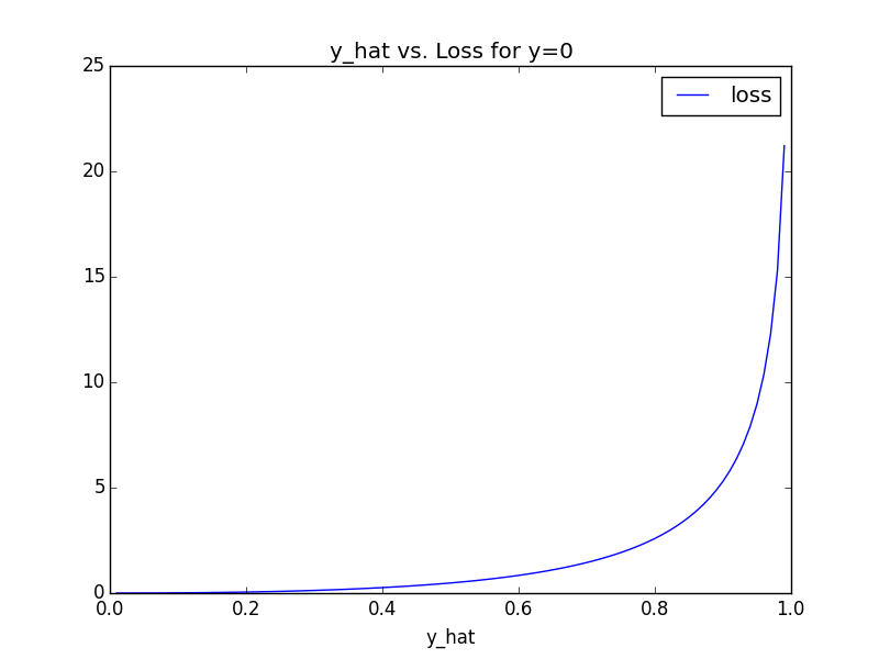
When \(y = 1\), our cost is that of the typical logarithmic loss. At worst, our cost is \(\approx 5\). However, when \(y = 0\), the dynamic is different: if we guess \(0.2\), it's not so bad; if we guess \(0.6\) it's not so bad; if we guess \(> 0.8\), it's really, really bad. \(\approx 25\) bad. Finally, we compute our gradient. As easy as:

gradient = grad(custom_loss_given_weights)

And, lastly, apply basic gradient descent:

for i in range(10000):
    weights -= gradient(weights) * .01

That's it. Implementing a custom loss function into your machine learning model with autograd is as easy as "call the grad function."

Why don't people use this more often?

Code:

All code used in this post can be found in a Jupyter notebook on my GitHub.