Greetings, all, and welcome to my new website! For those that know me, I am the increasingly lazy creator and curator of Will Travel Life - where I post stories, photos, and philosophical muse from a 2+ year backpacking and cycling trip around the world. For those that don't, it's a pleasure to have you at my journalistic side.
In this blog, I'll be posting on a variety of mathematics and machine learning topics. Many will have a travel flavor. In this post, we'll take a look at air travel and airports on my favorite continent: South America and the Falkland Islands.
Traveling by plane in South America is not particularly pragmatic nor affordable: the air network is relatively limited, and flights are therefore costly. Most travelers opt to take the bus instead. When flying to South America, you're likely to enter via one of its major international air hubs: Bogotá, Lima, Santiago, Buenos Aires or São Paulo, for example. Needless to say, these airports are major connecting points for intra-continental travel as well.
In addition to these big airports we'll have a series of, qualitatively speaking, "semi-big" airports, "small" airports, "super tiny single-runway Cessna Jet only" airports, etc. Perhaps we can be more explicit with our grouping? It's one thing to attempt to classify these airports into distinct groups by how many McDonald's each houses. It's another to use the data. Here, I'll attempt this classification using shortest path analysis and k-means clustering.
First, I grab a list of all worldwide flight routes from OpenFlights, current as of January 2012 and containing "59036 routes between 3209 airports on 531 airlines spanning the globe." We filter for South America and employ R's "igraph" package - a library dedicated to network analysis and visualization. I then produce a basic social network graph for all flights between Chile, Argentina and Paraguay merely for example - a visual of some of the data at hand and a testament to the graphical power of R.
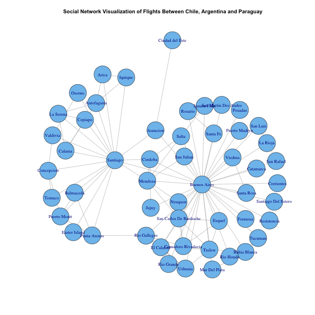
The simplify function is used to eliminate reverse routes: we don't need to map flights between Buenos Aires and Santiago as well as those from Santiago to Buenos Aires. As assumed, the visual confirms that most flights between these countries are done through the capitals: Buenos Aires, Santiago, and Asunción. Also, within Argentina, there appears to be a few "middle-range" airports as well, namely but not limited to Mendoza, Bariloche, and El Calafate. Clearly, there are countless "bottom-range" airports too serviced only by one city (within these three countries); Ciudad Del Este, for example. How many distinct groups of varying size/volume/connectivity can we form?
To answer this question, we compute the shortest path - or number of distinct airports through which one must fly - from every city in South America to all other cities. These values are then be used to inform centroid locations for our k-means analysis.
Unfortunately, we still must tell R how many clusters we seek. Should there be 4 distinct airport groups? 8? Why? The more clusters we have, the closer values within each cluster move to their respective centroid mean, a metric given by withinss or "within groups sum of squares." Therefore, we first run the analysis for varying numbers of clusters in search of the k value at which the "marginal return of adding one more cluster is less than was the marginal return for adding the clusters prior to that." We run trials for \(k = 2\) to \(k = 9\). The article "K-means Clustering 86 Single Malt Scotch Whiskies" on the Revolution Analytics blog was referenced heavily for this step.
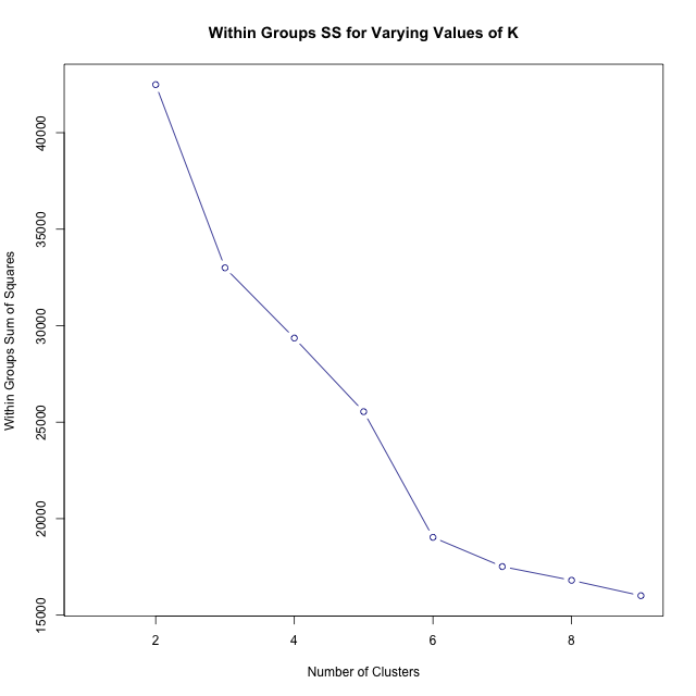
From the graph, it appears that \(k = 3\) is the value we want: "the marginal return of adding one more cluster is less than was the marginal return for adding the clusters prior to that." However, the k-means clustering algorithm does incorporate a random number generator, so it is important to examine the impact of randomness on our results. In addition, after producing this graph a few times, it was immediately clear that our trend varies slightly across trials. In solution, we'll run 100 trials in ggplot, plot them in points, and examine the smoothing line instead.
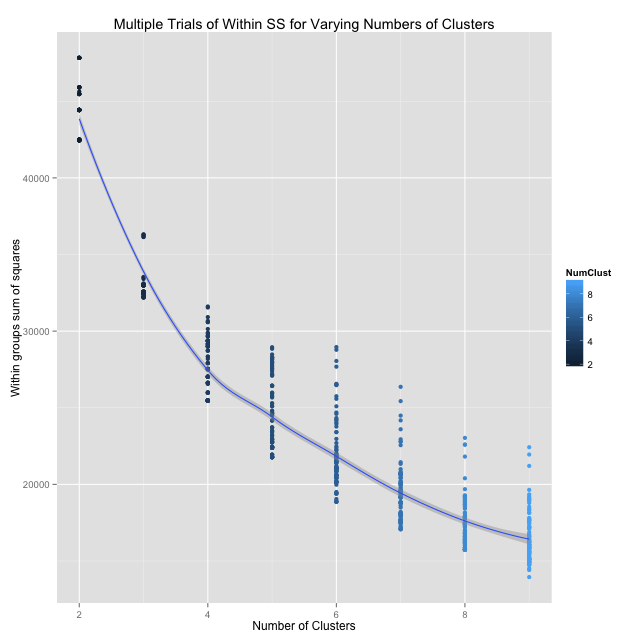
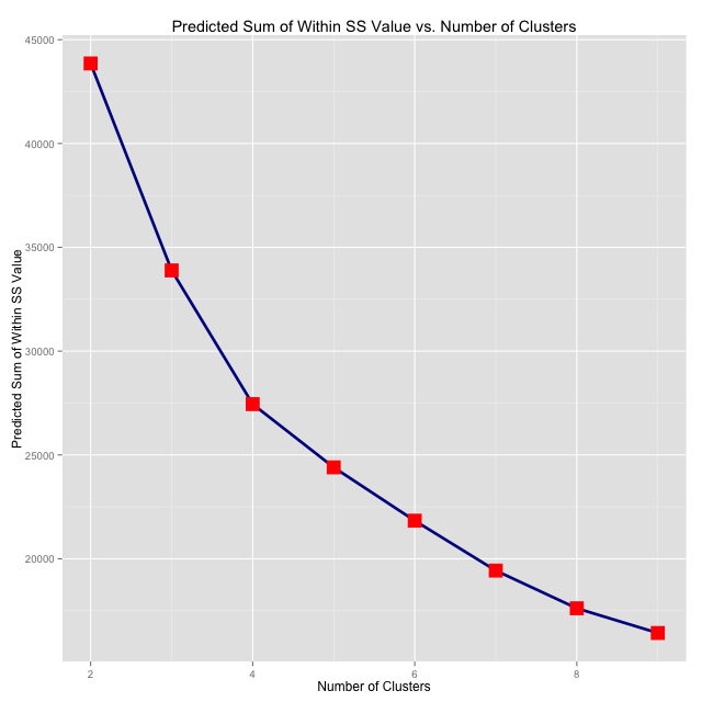
The plot seems to corroborate what we previously thought: \(k = 3\) clusters is the best choice for our data set. To be absolutely certain, we can explicitly compute the predicted "loess" values that fall on our smooth line for integers in \([2,9]\) and see where the "marginal returns cutoff point" really is. Simple subtraction.
PredSumVal K
1   43854.32 2
2   33887.51 3
3   27447.83 4
The graph shows the marginal returns clearly. And since \((43854.32 - 33887.51) \gt (33887.51 - 27447.83)\), our assumption is confirmed definitively. We want to choose \(k = 3\) clusters: there are three levels of size/volume/connectivity for airports in South America. In the next post, we'll delve deeper into what this analysis can help us learn about each country and the continent as a whole.